Methods
This methods page covers the main Bay Area Greenprint reporting tool. To read more about the Mitigation Wizard, check out the Mitigation Wizard Methodology Page.
Nature’s values and benefits
As a global biodiversity hotspot, the non-built environment provisions many benefits to residents of the Bay Area alongside its extensive biodiversity value. The natural and agricultural resource information in the Bay Area Greenprint highlights nature’s benefits s and provides a framework for interpretation of this information. The Greenprint provides a more transparent connection between the values and benefits of nature in the Bay Area and its seven million residents.
The Bay Area Greenprint is organized around nine of nature’s values and benefits:
- Food production
- Water supply
- Water quality
- Water hazard risk reduction
- Carbon storage & air quality
- Outdoor recreation
- Prioritized habitats
- Habitat connectivity
- Species and habitats that might require mitigation
A final category, Urban Greening, identifies the need for, and opportunities to, enhance the benefits of natural and agricultural lands within urban areas.
For each resource that contributes to a benefit or value, the Greenprint identifies the status of protection through fee, easement, or policy. Similarly, climate change intersects with nearly all of nature’s values posing possible threats and opportunities to the continued presence of the value.
Read more about the user-defined multi-benefit conservation assessment layers.
The Bay Area Greenprint recognizes the opportunities to bring environmental resources into our cities, known as Urban Greening, as well that nature can sometimes be a Hazard to the developed infrastructure.
Reporting Framework
Meaningful Interpretation of Natural Resource Accounting
The Greenprint produces individualized reports quantifying the natural and agricultural resources within a user-defined area of interest. The degree to which natural and agricultural resource information will influence decisions will require more than details about the quantity of a resource within an area of interest. Influence will require clear communication of the significance of that resource or of the quantity of that resource to a local area or to the region. In evaluating and communicating significance, the Greenprint seeks to answer the question: Does this quantity of this resource in this location matter?
To this end, the report provides:
- Quantity: The total quantity or value of each resource within the area of interest
- Relevance: Comparison of the quantity of a resource in an area of interest to the quantity in:
- The nine-county Bay Area (region)
- The county
- The watershed (local)
- Status of resource protection: The quantity of the resource on lands protected by easement or fee
- Regionally in the nine-county Bay Area
- In the county
- Did you know?: A key fact that further interprets this information (e.g. equivalencies) or additional information that makes this resource particularly beneficial or relevant (e.g. exists within a drinking water watershed)
- Policies: Relevant policies will be listed when they provide protection for that resource in that area
- Climate change: The Greenprint will reveal 1) the threat climate change poses to each relevant value or benefit, and 2) potential opportunities to protect that value or benefit, given a changing climate.
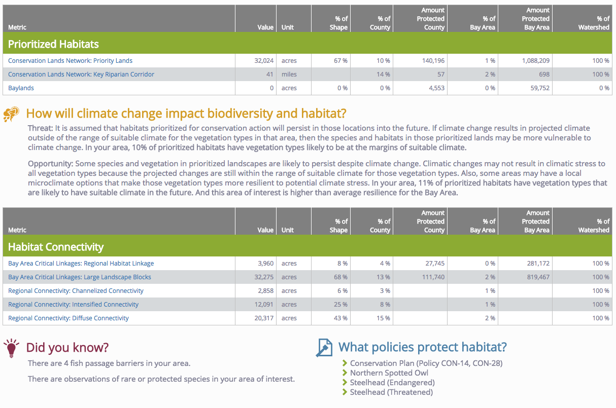
The figure below illustrates an example of the Greenprint report. The metric reporting, local and regional relevance, and protection status are listed in tabular format for each resource. Climate change and policy information and additional interpretations are called out below the tables when applicable.
Policies
Open space that surrounds the Bay Area’s urban core are covered by policy measures that vary in their efficacy at protecting natural or agricultural lands. Policies are collected from city and county plans, and regional, state, and federal agencies and assessed by the language that enforces the protection of or limits on urban development activity on conservation values, including agriculture, habitat, water resources, and our region’s precious bayland and coastal resources. Lands considered to have high policy protection are protected by one or more policy measures that prohibit most development. Lands considered to have medium policy protection are protected by one or more policy measures where development is intended to be limited but is still possible with a special permit. Lands considered to have low policy protection lands do not fall under any specific protective policy measures.
Climate Change
Climate change is one of the major global challenges facing biodiversity and human populations (CITE). The Bay Area is projected to get warmer and increasingly water-stressed. Climatic changes may be outside the range of historic variability or outside the range of suitable conditions for plants, animals, or crops in a given location causing stress to human-systems and nature. Even if changes are within the range of historic variability, climatic extremes, including droughts and floods, will become more common, further stressing biodiversity, agriculture, and water resources.
Threats from climate change include:
- inundation from sea-level rise and from increased frequency and extents of floods which could impact coastal and downstream urban populations, transportation infrastructure, and agriculture in the area,
- increased droughts which could impact groundwater supply,
- an increase in the irrigation needed to support current local crops, and
- stressed vegetation, species, and communities in habitats prioritized for biodiversity protection.
There are still opportunities to protect people and infrastructure from hazards by protecting and restoring natural infrastructure, to innovate and adapt agriculture to keep food production local to the Bay Area, to avoid development in areas that are particularly important for recharging aquifers, and to protect habitat in resilient areas or areas that are less likely to be stressed by climatic changes.
Urban Greening
Nature’s values and benefits traverse the imaginary boundary between open space and built up lands. Within cities, urban greening refers to public landscaping and urban forestry projects that create mutually beneficial relationships between city dwellers and their environments. The presence of green spaces can enhance the health and wellbeing of people living and working in cities by improving physical fitness, reducing depression and improving air quality. Thoughtfully designed green spaces also impact the financial efficiency of our cities, such as urban forestry limiting the impact of heatwaves by shading out our buildings or through keeping flood zones undeveloped as open space to help absorb stormwater flooding that may impact downstream homes and businesses.
Nature’s Values and Benefits Framework
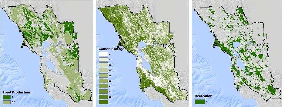
Agriculture
Food production
Description: Areas with land use, climate, soil type, and irrigation capacity (if applicable) to currently support the production of food through agriculture and ranching.
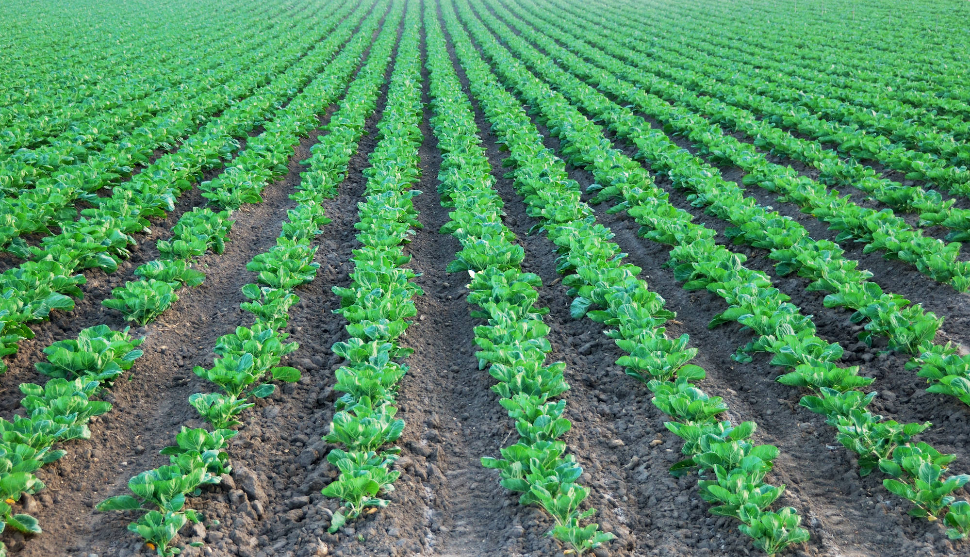
A field of collard greens, California. Photo by goldenangel, iStock.
Benefits: Food production (~$1.4 billion dollars in the Bay Area)
Benefit Recipients: Bay Area population and beyond
Metrics: Agricultural areas include the following areas with definitions from the Department of Conservation’s Farmland Mapping and Monitoring Program:
- Prime Farmland – Farmland with the best combination of physical and chemical features able to sustain long term agricultural production. This land has the soil quality, growing season, and moisture supply needed to produce sustained high yields. Land must have been used for irrigated agricultural production at some time since 2010.
- Farmland of Statewide Importance – Similar to Prime Farmland but with minor shortcomings, such as greater slopes or less ability to store soil moisture. Land must have been used for irrigated agricultural production at some time since 2010.
- Unique Farmland – Farmland of lesser quality soils used for the production of the State's leading agricultural crops. This land is usually irrigated, but may include non-irrigated orchards or vineyards as found in some climatic zones in California. Land must have been cropped at some time since 2010.
- Farmland of local importance – Land of importance to the local agricultural economy as determined by each county's board of supervisors and a local advisory committees.
- Grazing land – Land on which the existing vegetation is suited to the grazing of livestock.
Data Source: Farmland Mapping and Monitoring Program (FMMP).
Metric Unit: Acres of each FMMP category.
Method: Total acres of each FMMP category were summed for an area of interest.

Did you know that crops in this area are worth as much as $XX,000?
Data: County agricultural commissioner data cross-walked to and summarized by FVEG 2015 agricultural types.
Method: County agricultural commissioner crop types were cross-walked to the agriculture California Wildlife Habitat Relationship (CWHR) types in FVEG 2015 according to CWHR type descriptions. These cross-walk relationships are listed in this table. The production value per harvested acre was then averaged across crop types associated with each CWHR agricultural type within each county. If a CWHR type in a county had no associated crop production value in the county crop report, a statewide average production value was used for that CWHR type. Value per acre was then converted to total dollar value per 30m grid (equation 1).

Equation 1. Conversion of agricultural type value per acre to total production value of each grid cell
Production value was then summed across the area of interest.
 How will climate change impact food production?
Threats to food production in a changing climate
A warmer and/or drier climate may require additional irrigation to maintain the same crop in the same location.
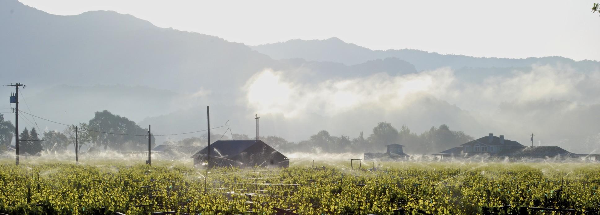
Irrigated cropland in Napa County. Photo by Craig Camp, CC-BY, Flickr.
Metric: Acre-feet of additional irrigation needed to offset climate change.
Data: Delta Climate Water Deficit (CWD) (USGS 2014) in locations where CWD is expected to increase. CWD quantifies evaporative demand exceeding available soil moisture and is measured in mm/yr. Projected increases in CWD in agricultural areas will indicate the additional water that may be needed at a given location to maintain status quo in terms of agricultural production.
Method: Global Circulation Models (GCM) project future climate conditions based on greenhouse gas concentrations and oceanic and atmospheric circulation. There is variation in climate projections across climate models (Figure 1) and across emission scenarios. A baseline emission scenario (Representative Concentration Pathway (RCP) 8.5) assumes high energy demand, no policies for climate change mitigation, and little technological improvements in the energy sector (Raihi et al. 2011). Historic and future modeled climate projections were downscaled to 270m (Flint & Flint (2012) and run through the Basin Characterization Model to derive hydrologic climate variables (Flint et al. 2013).
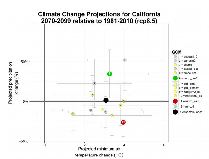
Figure 1: Reproduced with permission from ‘A climate change vulnerability assessment of California’s terrestrial vegetation’ (Thorne et al. 2016).
We used projections from three GCMs to represent the average change expected and the range of climatic changes that the Bay Area is likely to experience.
Additional irrigation needed to offset climate change was reported for the CCSM4 model which projects temperature and precipitation changes that approach the average change from 10 GCMs. The range in this metric was calculated as the potential minimum amount of additional irrigation needed to offset climate change from a warm and wet GCM (CNRM) and the potential maximum amount of additional irrigation needed to offset climate change using a hot and dry GCM (MIROC).
All projections were modeled for mid-century (average projections for the years 2040-2069) and used the baseline emissions scenario (RCP 8.5). Extensive policy changes and drivers of technological innovation would need to be in place to approach the RCP 4.5 scenario and were not included in this analysis.
Delta CWD was calculated by subtracting the historic average CWD for 1981-2010 from future CWD for the three climate models described above. All negative values were removed to evaluate only areas with projected increases in CWD as the additional irrigation that might be required in a given location to maintain the status quo. This resulted in three rasters representing the increases in CWD expected for three different climate models. Each layer was limited to just those areas that currently support agriculture or ranching identified in the FMMP as Prime Farmland, Farmland of Statewide Importance, Unique Farmland, Farmland of Local Importance or Grazing Land. These rasters of increases in CWD in agricultural lands were then converted from mm/yr to total volume of water in acre-feet with the following equation:

Equation 2: Conversion of Delta CWD in mm/yr to total volume of water.
Total volume was then summed within an area of interest for each of the three climate scenarios.
 What policies protect food production?
The following policies protect agricultural land in the Bay Area.
| Policy | Jurisdiction | Protection |
|---|---|---|
| Agricultural Conservation Area | Brentwood | Through the use of policies concerning the conversion of agricultural lands and the creation of buffer zones between agricultural and nonagricultural uses, it will be possible to conserve areas of agricultural land. |
| Briones Hills Agricultural Preservation Area | Contra Costa County, Martinez, Pleasant Hill, Walnut Creek, Lafayette, Orinda, Richmond, Pinole, and Hercules | The plan supports that no land will be added within the 64 square mile area in order to leave room for urban development. The plan also dictates that the area will stay in public and agricultural use during the planning period. |
| Measure C Agricultural Core | Contra Costa County | This land is designated to preserve and protect the County farmlands most capable of the production of food and fiber from Measure C in 1990. Its an attempt to maintain economically viable agricultural units while discourage "ranchette" housing development. |
| Agricultural Buffer Transition Area | Gilroy | Agricultural mitigation requires equal protection (1:1 ratio) for the loss of agricultural lands that no longer will be designated agricultural land due to conversion to urban uses and require a 150 foot buffer between new urban and agricultural uses. |
| South Livermore Valley Area Plan | Livermore | The plan seeks to protect, enhance, and increase viticulture and other cultivated agriculture in the South Livermore Valley, directing development away from potential agricultural land. |
| Agricultural Priority Area | Morgan Hill | Agricultural Priority Area identified as the Morgan Hill's first priority for conservation inside the city's sphere of influence. |
| Measure P Agricultural Lands Preservation Initiative | Napa County | Changes to the General Plan for minimum parcel size and maximum building intensity of lands designated for agriculture and watersheds cannot occur unless approved by the voters, with certain limited exceptions. |
| Measure T Orderly Growth Initiative | Solano County | The Orderly Growth Initiative focuses residential growth in the county's seven cities, rather than the unincorporated areas. Lands zoned for agriculture cannot change without a popular vote thereby supporting the County’s economy and quality of life. |
| Winters Agricultural Preserve | Solano County | Agricultural Reserve Overlay. |
| Agricultural Enterprise Area | San Mateo County | Privately owned lands meeting zoning designation and general land use criteria for eligibility under the Williamson Act for landowners considering entering into an Agricultural Preserve and Williamson Act contract, non-regulatory and non-obligatory. |
| Davis-Dixon Greenbelt | Dixon, Davis, the Solano Land Trust, federal and state agencies | Agricultural Reserve Overlay. Permanently protecting the prime farmlands and scenic resources of the area located between the two cities. |
| Vacaville-Dixon Greenbelt | Vacaville-Dixon Greenbelt Authority | Agricultural Reserve Overlay. Prioritize lands located between the two cities remain an agricultural landscape in perpetuity, implemented through acquisition from willing sellers and resale of the properties with a permanent conservation easement. |
| Williamson Act Properties with Ongoing Contracts | Alameda County, Contra Costa County, Marin County, Napa County, San Francisco, San Mateo County, Santa Clara County, Solano County, Sonoma County | California law that provides relief of property tax to owners of farmland and open-space land in exchange for a ten-year agreement that the land will not be developed or otherwise converted to another use. |
Methods: The jurisdictional policies adopted that prioritize agricultural conservation of natural resources and preservation of farms and ranches from urban development are reviewed and digitally rendered based upon jurisdictions’ general plans and zoning maps. Williamson Act property shapefiles are shared by Bay Area county conservation agencies from 2016 and Marin County from 2012. The shapefile filters out expiring Williamson contracts for owners opting out of the agricultural policy protection.
Biodiversity
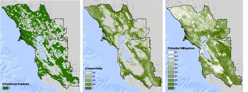
Prioritized Habitats
Description: Prioritized habitats for conserving biodiversity in the Bay Area, a global biodiversity hotspot.
Metrics: Prioritized habitats include priority uplands designated and defined by the Conservation Lands Network, key riparian corridors, and natural terrestrial baylands.
Conservation Lands Network (CLN): The CLN is made up of the lands that, if protected from development, can preserve the Bay Area’s upland biodiversity into the future.
Key Riparian Corridors: Streams prioritized to maintain healthy assemblages of native fish.
Natural terrestrial baylands: Due to the high rate of conversion of wetland habitat, all remaining wetlands are considered prioritized habitat. The CLN includes upland wetlands, but excludes baylands. Therefore, all remaining natural terrestrial baylands complement the CLN.
Data:
- Conservation Lands Network
- Key Riparian Corridors
- Natural terrestrial baylands
Metrics:
- Total acres of prioritized upland habitat summed across the three categories
- Miles of key riparian corridors
- Total acres of natural terrestrial baylands
Methods:
- Habitats classified as Essential, Important, and Fragmented (priority habitats fragmented by development) in the Conservation Lands Network were combined into a single data layer representing the CLN-prioritized uplands. Acres of CLN priority areas were summed in an area of interest.
- Key riparian corridors were limited to just Priority 1 and Priority 2. Total miles of riparian corridors were summed in an area of interest.
- Natural terrestrial baylands were limited to just those that were both terrestrial and naturally formed. Acres of natural terrestrial baylands were summed in an area of interest.
How will climate change impact prioritized habitats?
Threats to prioritized habitats in a changing climate
It is assumed that areas prioritized for conservation action will have habitats and species that persist in those locations into the future. If climate change results in projected climate conditions at the margins of or outside of the range of suitable climate for the vegetation types in that area, then vegetation may be stressed and the species and habitats in those prioritized lands may be more vulnerable to climate change.
[Insert image of stressed vegetation in Bay Area]
Drought stressed tree in California, photo credit: xx
Metric: Percent of prioritized habitats with vegetation types that are likely to be at the margins or outside of suitable climate conditions
Data: Thorne et al. analyzed projected climate exposure for each of the 64 CWHR types from FVEG 2015. If less than 5% of the extent of that vegetation type in California currently experiences the climate conditions that are projected in that area, then the vegetation in that area was considered to be exposed.
Method: Levels of CWHR type vegetation exposure from mid-century projections and baseline emissions (RCP 8.5) for a hot and dry scenario (MIROC) and a warm wet scenario (CNRM) were modeled to bracket the degree of exposure expected from the range of projected changes in climate in California (Figure 1).
Results were limited to just the areas with >95% exposure for both climate scenarios. This intersection gives more certainty to the estimates of stressed vegetation because these areas are projected to be stressed regardless of the range of different projections of climate change. The stressed vegetation types were then limited to only lands classified as natural land using FVEG 2015 resampled to 270m, and to only the upland habitats that were prioritized by the CLN as essential, important, or fragmented. The result was summed for the area of interest and reported as the percent of stressed vegetation of all natural land in prioritized habitats.

Opportunities for prioritized habitats given a changing climate
For some habitats, climatic changes may not result in climatic stress to vegetation types because the changes are still within the suitable climate for those vegetation types. Also, some areas may have a diversity of accessible microclimate options so that even if climatic changes at a coarser scale are projected to stress vegetation, there will likely be local opportunities available where those species and habitats can access suitable climate, making those prioritized areas more resilient to climate change. Areas where vegetation will be less stressed or areas with higher resilience are areas where habitats and biodiversity are more likely to persist in place despite climate change. Therefore, areas that are prioritized for conservation action based on the species and habitats they currently support, that are more likely to continue to support those species and habitats in the future, will likely still be priorities for biodiversity even in a changing climate.
[Insert image of local microclimates resulting from differences in aspect]
local microclimates resulting from differences in aspect, photo credit: xx
Metrics:
- Percent of prioritized habitats with vegetation types that are likely to still have suitable climate in the future
- Resilience score (i.e., this area of interest is higher than average resilience for the Bay Area)
Data:
Thorne et al. analyzed climate exposure for each of the 64 CWHR types from FVEG 2015. A vegetation type in an area was considered not to be exposed if future climatic conditions were projected to be within the range of climate conditions that 80% of that vegetation type currently experiences in California.
Landscape Resilience (TNC) is a combined measure of topoclimatic diversity and local permeability, providing an indicator of availability of accessible microclimate options. Topoclimatic diversity is measured for a 157-acre neighborhood using a 450m moving window for each 90m gridcell to describe the range in ‘heat’ (HLI – Heat Load Index) and the range in ‘wetness’ (CTI – Compound Topographic Index). More diversity in heat and wetness means more locally cooler or wetter areas exist near hotter and drier areas, providing more options for species to redistribute locally to find suitable climate. Permeability is measured as the proportion of the landscape within 3km that a species is able to access without encountering significant barriers to movement from anthropogenic land uses. Permeability is combined with topoclimatic diversity to address the accessibility of available microclimates.
Methods:
- Levels of CWHR type vegetation exposure from mid-century projections and baseline emissions (RCP 8.5) for a hot and dry scenario (MIROC) and a warm wet scenario (CNRM) were modeled (Thorne et al. 2016) to bracket the degree of exposure expected from the range of projected changes in climate in California (Figure 1). Results were limited to just the areas with <80% exposure for both climate scenarios. This intersection gives more certainty to the estimates of vegetation unlikely to be stressed by climate change because these areas are projected to be within the range of climate suitable for that vegetation type in California regardless of the range of different projections of climate change. These unstressed vegetation types were then limited to only lands classified as natural land using FVEG 2015 resampled to 270m, and to only the upland habitats that were prioritized by the CLN as essential, important, or fragmented. The result was summed for the area of interest and reported as the percent of vegetation unlikely to be stressed by climate change of all natural land in prioritized habitats.
- We rescaled the resilience index data into 100 equal bins ranging between 0.01 and 1. The average resilience score was calculated within an area of interest and compared to the average resilience score across the Bay Area.
What policies protect prioritized habitats?
The following policies protect prioritized habitat land in the Bay Area.
| Policy | Jurisdiction | Protection |
|---|---|---|
| Altamont Pass Wind Resource Area | U.S. Fish & Wildlife Service, Alameda County, Contra Costa County | The Altamont Pass Wind Resources Area Conservation Plan is being developed to minimize impacts to birds caused by wind turbines, and conserve birds and other terrestrial species while allowing wind energy development and operations in the area. |
| Bay/Delta Conservation Plan NCCP/HCP | California Department of Water Resources, U.S. Bureau of Reclamation | The Plan goals are to provide for the conservation and management of endangered and threatened species through habitat preservation and restoration as well as streamline environmental permitting process for water projects and some development. |
| East Contra Costa County NCCP/HCP | Brentwood, Clayton, Oakley and Pittsburg, Contra Costa County, Contra Costa County Flood Control and Water Conservation District and East Bay Regional Park District | The East Contra Costa County HCP/NCCP is intended to provide regional conservation and development guidelines to protect natural resources while improving and streamlining the permit process for endangered species and wetland regulations. |
| San Bruno Mountain Area HCP | San Mateo County | San Bruno Mountain Area HCP is a way to protect and improve habitat for an endangered species in conjunction with limited development on San Bruno Mountain. |
| Santa Clara Valley NCCP/HCP | Santa Clara Valley Habitat Agency: Gilroy, Morgan Hill, San José, Santa Clara County, Santa Clara Valley Water District, and Santa Clara Valley Transportation Authority | A primary goal of HCP is to obtain authorization for incidental take of covered species under the ESA and the NCCP Act for covered activities which will occur in accordance with approved land-use and capital-improvement plans. |
| Solano Multi-Species HCP | Solano County Water Agency, Vacaville, Fairfield, Suisun City, Vallejo, Solano Irrigation District, Maine Prairie Water District | The Solano HCP establishes a framework for complying with endangered species regulations while accommodating future urban growth, development of water-related and other public infrastructure undertaken by the Plan Participants. |
| Stanford HCP | Stanford University | The Stanford HCP establishes a comprehensive conservation program that protects, restores and enhances habitat areas; monitors and reports on covered species populations; and avoids and minimizes impacts on species and their habitats. |
| Sonoma County Biotic Habitat designation | Sonoma County | Protection of these areas helps to maintain the natural vegetation, support native plant and animal species, protect water quality and air quality, and preserve the quality of life, diversity and unique character of the County. |
| Santa Rosa Plain Conservation Strategy Study Area | U.S. Fish & Wildlife Service, Alameda County, Contra Costa County | Create a long-term conservation program sufficient to mitigate potential adverse effects on listed species due to development on the Santa Rosa Plain. |
Methods: The jurisdictional policies adopted that reduce impacts on priority habitats from urban development are reviewed and digitally rendered based upon jurisdictions’ general plans and shared or download from Habitat Conservation Plan agencies.
Biodiversity
Habitat Connectivity
Connectivity enhances biodiversity values by supporting gene flow between populations and enhancing adaptation of biodiversity to climate change by facilitating range shifts.
Metrics:
- Focal Species Connectivity, Bay Area Critical Linkages
- Focal Species Connectivity, Large Landscape Blocks
- Regional Connectivity, Channelized: Last remaining natural linkages through a region
- Regional Connectivity, Intensified: One of few remaining natural options for regional movement
- Regional Connectivity, Diffuse: Broad, unfragmented lands, important to regional movement
- Metric Units: Acres of each class
- Acres of important areas for focal species regional connectivity
- Acres of important areas that contribute to regional connectivity
Data:
- Bay Area Critical Linkages and associated natural landscape blocks (Critical Linkages: Bay Area and Beyond, 2013)
- Regional Connectivity – Omniscape (TNC 2017)
Methods:
- Bay Area Critical Linkages (http://www.scwildlands.org/reports/CriticalLinkages_BayAreaAndBeyond.pdf) is a network of habitat linkages designed for a number of focal species using least-cost path modeling to connect large intact areas across suitable habitat. Acres within a linkage are summed and reported in an area of interest.
- Omniscape regional connectivity for California represents a wall-to-wall picture of regional habitat connectivity for plant and animal species whose movement is inhibited by developed or agricultural land uses. The approach uses a modified version of Circuitscape (http://www.circuitscape.org/) with a moving-window algorithm to quantify ecological flow (potential connectivity) among all pixels within a 50km radius. Circuitscape treats landscapes as resistive surfaces, where high-quality movement habitat has low resistance and barriers have high resistance. The algorithm incorporates all possible pathways between movement sources and destinations and identifies areas of high flow via low-resistance routes (i.e., routes presenting relatively low movement difficulty because of lower human modification, and thus mortality risk). Omniscape output was limited to just channelized (last remaining natural linkages through a region), intensified (one of few remaining natural options for regional movement), and diffuse (broad, unfragmented lands, important to regional movement) connectivity classes, condensed across all levels of flow, and summarized by acres of each class in an area of interest.
Did you know your area of interest contains X barriers to fish passage?
Did you know your area if interest contains a linkage with a pinch point?
Data:
- Fish passage barriers
- Pinch points in critical linkages across highways
Methods: The area of interest was screened for the presence or absence of fish passage barriers and separately for the presence or absence of a critical linkage that has a pinch point within a half mile of the area of interest.
What policies protect habitat connectivity?
The following policies protect habitat connectivity in the Bay Area.
| Policy | Jurisdiction | Protection |
|---|---|---|
| Sonoma County Open Space Habitat Connectivity Corridors | Sonoma County | Habitat Connectivity Corridors are areas where property owners are encouraged to promote wildlife friendly modifications to their property such as the installation of wildlife friendly fencing; includes Sonoma Valley Corridor and Laguna West Corridor. |
Methods: This jurisdictional policy addressing habitat connectivity is downloaded from Sonoma County Permit Resource and Management Department.
Biodiversity
Species and habitats that might require mitigation
Knowledge of the locations of threatened and endangered species habitat and protected habitats helps identify areas where development could lead to costly mitigation and provides efficient mitigation opportunities for development projects.
Benefits: Cost savings and efficiencies in development projects due to early identification, and potential avoidance, of impacts to species or habitats that require mitigation and the conservation of ample future mitigation opportunities.
Benefit recipients: Transportation agencies and developers
Metrics:
- Hotspots of species requiring mitigation: 167 threatened and endangered species in the Bay Area could be impacted by proposed transportation projects over the next 20 years. If impacted, these species would require take permits and mitigation. Hotspots of habitat that that may require mitigation provides an early, rough estimate of where there could be impacts to listed species enabling an early assessment of potential permit requirements and mitigation needs for a project, the opportunity to avoid impacts early in the planning process, and identification of possible mitigation sites. This data indicates the cumulative hectares of suitable habitat in a 25 hectare region for species that may be impacted by proposed transportation projects in the next two decades.
- Habitat value for threatened and endangered species:
- Wetlands: Saturated habitat that supports specially adapted plants and animals. Because 85% of the historic wetlands have been converted or altered, many policies are in place to protect wetlands.
- Vernal Pools: Type of wetland with low surface water runoff that fill during the rainy season then desiccate from evapotranspiration, forming a unique habitat with specialized amphibians and insects
Data:
- Huber et al. 2013 identified species likely to be impacted by planned transportation projects. Observation recorded in the California Natural Diversity Database (CNDDB) were buffered to two and four miles and screened for vegetation types (CWHR types) that provided highly suitable habitat for those potentially impacted species within the buffers. These were considered habitats likely to support species that may require mitigation from transportation projects. Total cumulative habit for all species in both buffers was summed across 25 hectare hexagons.
- CWHR types were cross-walked to average habitat suitability scores across all life history classes and all size and structure classes for ~62 threatened and endangered terrestrial vertebrates (mammals, birds, reptiles, amphibians). The urban class was subdivided into two classes: 1) a class with no tree canopy or an impervious surface, and 2) a class with high tree canopy and/or a high percentage of surface that was not impervious. These classes were assigned 0 suitability for all species or the CWHR average urban suitability score for each species respectively. All suitability scores for each species were clipped to the range of that species and then summed across all species and ranges.
- Wetlands include federal and regional sources and summed for total wetland acres. The Fish and Wildlife service include the wetland types, 'Estuarine and Marine Wetland', 'Freshwater Emergent Wetland', and 'Freshwater Forested/Shrub Wetland. The San Francisco Estuary Institute’s Bay Area Aquatic Resource Inventory V2 include wetlands types as 'Depressional' and 'Playa'.
- Vernal pools include federal and regional sources and summed for total vernal pool acres. The CA Department of Fish and Wildlife includes the Vernal Pool Complexes of the Central Valley from 1989-1998 [ds36] identified as 'High Density', 'Medium Density', 'Medium Density Disturbed', 'Low Density', and 'Low Density disturbed'. The San Francisco Estuary Institute’s Bay Area Aquatic Resource Inventory V2 include wetlands types as 'Vernal Pool'.
Methods:
- Area weighted averages were taken across the hexagons or portions of hexagons in an area of interest and classified according to the following divisions:
- None
- 1-25 hectares: Some habitat that supports one to a few species that may require mitigation from transportation infrastructure
- 26-50 hectares: Habitat supports some species that may require mitigation from transportation infrastructure
- 51-100 hectares: Habitat supports many species that may require mitigation from transportation infrastructure
- 101-Max hectares: Hotspot of habitat for species that may require mitigation from transportation infrastructure
- Habitat value for threatened and endangered species:
- Wetlands: Acres were summed for all wetlands in an area of interest
- Vernal Pools: Acres were summed for all vernal pools in an area of interest
In your area of interest there were observations of rare or protected species.
Data: CNDDB
We filtered CNDDB extant species observations to occurrences accurate to at least 1/10 of a mile, after 1990 for species that are either Species of Special Concern, State or Federally Threatened, Endangered, or candidates, or considered rare (i.e., rare plant, or state or Federally-ranked rarity S1-3 or G1-3).
What policies protect species and habitats that might require mitigation?
The following policies protect habitat connectivity in the Bay Area.
| Policy | Jurisdiction | Protection |
|---|---|---|
| Critical Habitat | Alameda County, Contra Costa County, Marin County, Napa County, San Francisco, San Mateo County, Santa Clara County, Solano County, Sonoma County | Areas identified as essential for the conservation of a threatened or endangered species under the Federal Endangered Species Act that may require special management and protection. |
Methods: The Critical Habitat designated areas are based upon (date - Jan 2016) data and are available for download from U.S. Fish and Wildlife Service Critical Habitat Portal (http://criticalhabitat.fws.gov/crithab/).
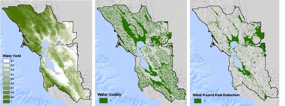
Water Resources
Water Supply
Total water supply indicates the contribution of the landscape to water supply by quantifying remaining precipitation after evapotranspiration that is available to surface water via runoff or to groundwater aquifers via recharge.
Benefit: Availability of water for agricultural water use and for drinking water through the replenishment of water in groundwater basins and surface water streams, lakes, and reservoirs.
Benefit Recipients: Water users (municipal and from wells) and farmers and ranchers.
Data:
- Groundwater Recharge: Water that infiltrates the into soils and aquifers
- Runoff: Water that flows over the land surface and feeds lakes, rivers, and streams
Metric: Acre-feet of water
Methods:
Recharge
Recharge is the historic 30-year average of recharge between 1981-2010. 270 meter cells and the value in each cell is an average rate of recharge (mm/year). To find the total volume of recharge (acre-feet) in a year for a different cell size, use the following equation:

Equation 5
Enter in the current rate value for x and the desired cell size in the 3rd step. If the cell size is not changing, remove the 3rd step from the equation.
Runoff
The raster dataset currently has 270 meter cells and the value in each cell is an average rate of runoff (mm/year). To find to total volume of runoff (acre-feet) in a year for a different cell size, use the following equation:

Equation 6
Did you know?

Equivalency
Did you know that XX acre-feet of groundwater recharge is equivalent to the annual water use for XX households?
Did you know that your area of interest intersects with X acres of watersheds that supply municipal drinking water?
Data:
- Municipal drinking water supply watersheds
- Reservoir catchment basins
- California Statewide Groundwater Elevation Monitoring (CASGEM) Groundwater Basin Prioritization
How will climate change impact water supply?
Threats to water in a changing climate
Climate change will likely change precipitation and evapotranspiration rates, impacting water supply by altering the quantity of water available for recharging groundwater and runoff to surface water. The Bay Area is likely to experience more extreme weather events including more frequent droughts.
Data: Basin Characterization Model (BCM) 2014 (USGS) number of years recharge + runoff are expected to exceed the tenth and ninetieth percentiles of historic variability.
Opportunities for water supply given a changing climate
With potential decreases in water supply and increases in water demand as the region becomes hotter and drier, and droughts become more frequent, groundwater basins will be increasingly stressed. Maintaining the infiltration potential of areas with soil and geologic conditions that are most suitable for direct aquifer recharge will become increasingly important in a changing climate.
Metric: Acres important for groundwater recharge
Data: Hydrogeologically vulnerable areas
What policies protect water supply?
The following policies protect water supply in the Bay Area.
| Policy | Jurisdiction | Protections |
|---|---|---|
| Sonoma County marginal groundwater area (Zone 3) | Sonoma County | Require proof of groundwater with sufficient yield and quality to support proposed uses in Class 3 water areas, test wells may be required, must demonstrate proposed use will not cause or exacerbate overdraft condition in groundwater basin or subbasin. |
| Sonoma County low/highly variable water yield area groundwater area (Zone 4) | Sonoma County | Require proof of groundwater with sufficient yield and quality to support proposed uses in Class 4 water areas without causing or exacerbating overdraft condition in groundwater basin or subbasin, require test wells or community water systems. |
Methods: This jurisdictional policy addressing water yield is downloaded from Sonoma County Permit Resource and Management Department.
Water Resources
Water quality
Areas where natural habitat provides a filtration benefit for surface runoff that maintains or improves surface water quality or where natural habitat provides a buffer for avoiding potential contamination of groundwater aquifers.
Benefit: Clean surface water; especially those that provide water to municipal water districts, clean runoff entering the bay, and avoided contamination of groundwater.
Benefit Recipients: Municipal water districts, farmers and ranchers, and urban populations.
Important areas for water quality include:
- Riparian buffers: Natural land cover within the Active River Area. Degraded catchments could otherwise be a source of sediment or pollutants into surface water, but natural land cover in the material contribution areas to a river provides a buffer to lessen the impact of these inputs from runoff. Riparian buffers within drinking water watersheds or reservoir basin catchments may be particularly important because there is a direct link between the benefit these natural lands provide to water quality of municipal drinking water
- Wetlands: Wetlands hold and filter pollutants and sediment before they are consumed into surface water. Wetlands within drinking water watersheds or reservoir basin catchments may be particularly important because there is a direct link between the benefit these wetlands provide to water quality of municipal drinking water.
- Baylands: Baylands with natural land cover help filter water from developed and agricultural uplands so that water entering the bay has reduced pollutants and sediment.
- Hydrogeologically vulnerable areas: These are areas where groundwater is susceptible to contaminants released at the surface. Natural land cover provides a benefit to groundwater quality by providing protection on the surface of these vulnerable regions by decreasing the likelihood of contaminant release in these areas through the avoidance of commercial activity.
Metric: Acres reported for each feature important to maintaining and improving water quality
Data:
- Natural land cover within Active River Areas
- Wetlands
- Natural baylands
- Hydrogeologically vulnerable areas
Methods:
- Land within the Active River Area was divided into natural and anthropogenic classes as determined by the National Land Cover Database (NLCD 2011). Natural classes were NLCD code: 11, 12, 31, 41, 42, 43, 51, 52, 71, 72, 73, 74, 90, 95 and anthropogenic classes were NLCD codes: 21, 22, 23, 24, 81, 82. Acres of natural lands in the Active River Area were summed.
- Wetlands include federal and regional sources and summed for total wetland acres. The Fish and Wildlife service include the wetland types, 'Estuarine and Marine Wetland', 'Freshwater Emergent Wetland', and 'Freshwater Forested/Shrub Wetland. The San Francisco Estuary Institute’s Bay Area Aquatic Resource Inventory V2 include wetlands types as 'Depressional' and 'Playa'.
- For natural baylands, land within the inundation zone of a sea level rise and storm event scenario (50 cm of sea level rise, 100-year storm) was divided into just the natural and semi-natural types as determined by the NOAA Coastal Change Analysis Program (see table below) and summed for total baylands acres.
- Hydrogeologically vulnerable areas were summed for acres in the area of interest.
|
Natural baylands land cover types (CCAP) (Listed in order of prevalence) |
Estuarine Emergent Wetland, Palustrine Emergent Wetland, Cultivated, Unconsolidated Shore, Grassland, Estuarine Aquatic Bed, Bare Land, Estuarine Scrub/Shrub Wetland, Palustrine Scrub/Shrub Wetland, Scrub/Shrub, Palustrine Forested Wetland, Evergreen Forest, Mixed Forest, Estuarine Forested Wetland, Deciduous Forest |
| Semi-natural baylands land cover types | Cultivated, Pasture/Hay |
Did you know that your area of interest contains X miles of a Clean Water Act Section 303(d) listed stream?
Did you know that your area of interest is within watersheds with water quality in the X percentile for the Bay Area?
Did you know that x% of your area is in a drinking water source watershed?
Data:
- California Integrated Assessment of Watershed Health Water Quality Index
- Clean Water Act Section 303(d) listed streams
- Drinking water source watershed
Methods:
- The water quality index was rescaled from statewide percentiles into percentiles for the extent of the Bay Area. This percentile value was averaged for the area of interest.
- California State Water Resources Control Board accounts for 2010 impaired water bodies. This shows the Clean Water Act Section 303(d) impaired water bodies of the 2010 Integrated Report’s list of combined categories 4a, 4b,and 5 with potential pollutant sources.
- Drinking water source watersheds were merged into a single layer and acres were summed and divided by the total area of the area of interest.
What policies protect water quality?
The following policies protect water quality in the Bay Area.
| Policy | Jurisdiction | Protections |
|---|---|---|
| Delta Primary Zone | Delta Protection Commission | Delta Protection Act is a policy to protect primary and secondary zone of delta the State to recognize, preserve, and protect those resources for the use and enjoyment of current and future generations. |
| Measure P | Napa County | Measure P extends the provisions of Measure J, the Agricultural Lands Preservation Initiative, which voters passed in 1990 to 2058. Specifically it continues to require voter approval for land designation changes in agricultural and watershed areas. |
| Measure T Orderly Growth Initiative | Solano County | It is an amendment to the 1994 orderly growth initiative to update certain provisions of the general plan land use and circulation element relating to agriculture or open space policies and land use designations and to extend the amended initiative. |
| Sonoma County Open Space Marshes Wetlands | Sonoma county | Preserve and restore freshwater marsh habitat of the Laguna de Santa Rosa area, the extensive marsh areas along the Petaluma River, another tidal marshes, and freshwater marshes such as the Pitkin, Kenwood, Cunningham, and Atascadero Marshes. |
| Suisun Marsh Protection Area - Primary Management Area | San Francisco Bay Conservation and Development Commission and the Department of Fish and Game | Existing uses within primary management area (managed wetlands, tidal marshes, lowland grasslands and seasonal marshes) should continue and both land and water areas should be protected and managed to enhance the quality and diversity of the habitats. |
| Suisun Marsh Protection Area - Secondary Management Area | San Francisco Bay Conservation and Development Commission and the Department of Fish and Game | Secondary management area should be act as a buffer area insulating the habitats within the primary management area from adverse impacts of urban development and other uses and land practices incompatible with preservation of the Marsh. |
| Coastal Zone | CA Coastal Commission | The Coastal Zone program manages the variety of planning, permitting, and non-regulatory mechanisms to manage its coastal resources, including issuing coastal development permits and reviewing local governments’ Local Coastal Programs. |
| San Francisco Bay Plan | San Francisco Bay Conservation and Development Commission | SF BCDC oversees the SF Bay and the surrounding shoreline, salt ponds, managed wetlands, and certain waterways in order to protect the Bay as a great natural resource for the benefit of present and future generations as well as develop the Bay and its shoreline to their highest potential with a minimum of Bay filling. |
Methods: The jurisdictional policies adopted that reduce impacts on water quality from urban development are reviewed and digitally rendered based upon jurisdictions’ general plans and or selected from protected zoning types from county zoning shapefiles.
Water Resources
Water hazard risk reduction
Natural lands can serve as natural infrastructure to reduce the risks from flood water and storm surges to urban areas and agricultural lands by reducing flood velocity, depth, and longevity.
Benefit: Reduced flood risk to cities and agricultural lands downstream.
Benefit Recipients: Population centers along shorelines in downstream floodplains.
Metric: Percent of X acres of floodplain or baylands are natural (e.g. 60% of 10 acres of floodplain are natural lands).
Data:
- Natural baylands
- Natural and agricultural land in the 100-year floodplain
- Peak Flow Retention, created from:
- Estimation of Direct Runoff from Storm Rainfall (NRCS 2004)
- Annual average precipitation (1981-2010 raw data from PRISM, downscaled for the California Basin Characterization Model
- Hydrologic soil groups: USDA Web Soil Survey
- Land Use and Land Cover (LULC, 2010 Coastal Change Analysis Program or C-CAP, from NOAA)
- Retention ratios database (Hamel et al., 2019)
- 100-yr return design storm (~40.4 mm): based on Intensity-Duration-Frequency curves for Redwood City
Methods:
- For natural baylands, land within the inundation zone of a sea level rise and storm event scenario (50 cm of sea level rise, 100-year storm) was divided into just the natural and semi-natural types as determined by the NOAA Coastal Change Analysis Program (CCAP) (see table below) and summed for total acres.
- For natural and agricultural land with the 100 year floodplain, the NLCD 2011 (2014) was clipped to the 100-year floodplain boundary (FEMA). Natural, agricultural, and urban land was classified as NLCD codes: 11, 12, 31, 41, 42, 43, 51, 52, 71, 72, 73, 74, 90, 95, NLCD codes: 81, 82, and NLCD codes 21, 22, 23, 24, respectively. Both natural and agricultural lands contribute to flood risk reduction downstream so both categories were included.
-
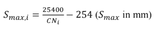
Flood retention was calculated for 16 urban classes, unique combinations of 4 types of urban LULC (low, medium, high intensity, and open space), and 4 soil types (hydrologic groups A to D, corresponding to decreasing infiltration rates). For each category i, stormwater runoff Qp (mm) is estimated with the Curve Number method:
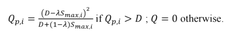 where D is the design storm depth in mm, Smax, i is the potential retention in mm, and λSmax is the rainfall depth needed to initiate runoff, also called the initial abstraction (λ=0.2 for simplification). Smax is related to the curve number, CN, an empirical quantity that depends on land use and soil characteristics (NRCS 2004):
 To calculate the design storm depth, we used intensity-duration-frequency (IDF) tables available for Redwood city, used as a representative area. The storm duration is equal to the average time of concentration of the studied watersheds, estimated at around 2 hours for small watersheds in the San Francisco Bay.
Based on the IDF curves, this corresponds to a 100-year return design storm of 40.4 mm. Some watersheds have larger times of concentration, but the goal of this layer is to compare flood reduction across the Bay Area, so the choice of the design storm can be subjective.
Flood retention in percentage (RQ) and volume (RQ,vol, in m3 ) is then calculated as:
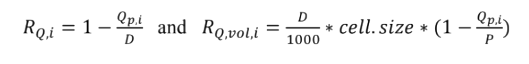 where cell size is the pixel area in m2.
Note: The modeling approach does not allow the quantification ofthis risk since only the on-pixel retention is calculated, without routing the floodwaters downstream.
References:
NRCS-USDA. (2004). Chapter 10. Estimation of Direct Runoff from Storm Rainfall. In United States Department of Agriculture (Ed.), Part 630 Hydrology. National Engineering Handbook. http://www.nrcs.usda.gov/wps/portal/nrcs/detailfull/national/water/?cid=stelprdb1043063: United States Department of Agriculture.
|
Natural bayland land cover types (CCAP) (Listed in order of prevalence) |
Estuarine Emergent Wetland, Palustrine Emergent Wetland, Cultivated, Unconsolidated Shore, Grassland, Estuarine Aquatic Bed, Bare Land, Estuarine Scrub/Shrub Wetland, Palustrine Scrub/Shrub Wetland, Scrub/Shrub, Palustrine Forested Wetland, Evergreen Forest, Mixed Forest, Estuarine Forested Wetland, Deciduous Forest |
| Semi-natural baylands land cover types | Cultivated, Pasture/Hay |
How will climate change impact water hazard risk reduction?
Threat: water hazard risk in a changing climate
Climate change may increase the frequency and extent of potential floods through sea level rise, increased storm surges, and increased flood frequency and intensity.
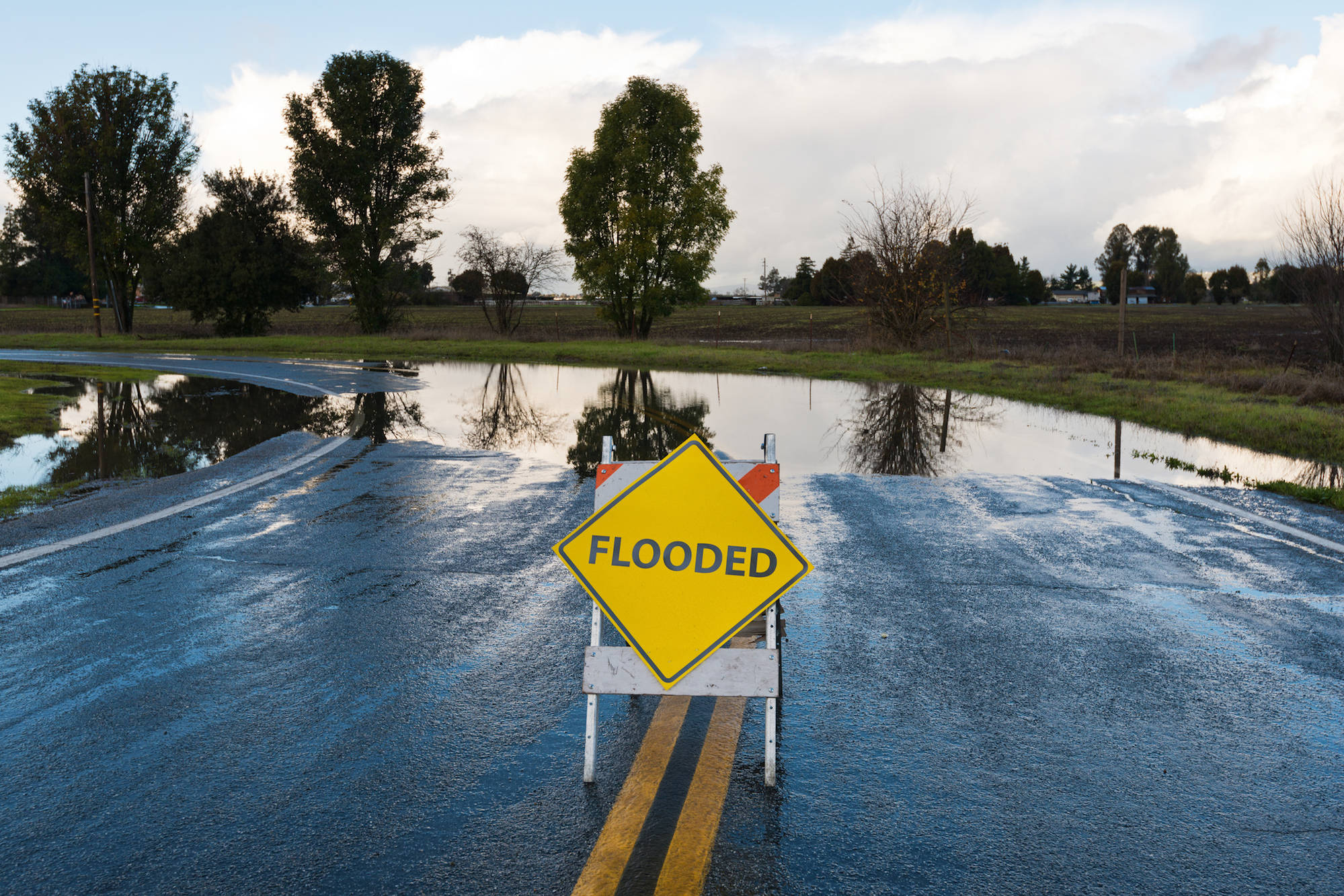
Flooded California road. Credit: Disorderly, iStock
Metrics:
- Percent of area of interest in projected sea-level rise inundation
- Percent of area of interest within the 500-year floodplain
Data:
- Sea level rise (Our Coast, Our Future, USGS) [50 cm + 100-year storm event]
- 500-year floodplain (FEMA)
Methods:
- The Greenprint Science and Methods Advisory Group agreed that an appropriate sea level rise scenario for 2050, the implicit planning horizon for the Greenprint, would be 50 cm. Since coastal hazards of sea level rise are exacerbated by storms (flooding and storm surge), it was agreed that the addition of a 100-year storm event would improve the characterization of water-related threat. The Our Coast, Our Future interactive Flood Map was used to generate the sea level rise/storm surge scenario.
- FEMA flood hazard data was limited to the 500 year extent (0.2% annual chance of flood). Because floods may be more frequent and more intense as a result of climatic changes, the 500 year floodplain may be inundated with more frequency than a 0.2% annual probability) and therefore development, agriculture, and infrastructure may have an increased risk of inundation in these areas.
Opportunities for water hazard risk reduction given a changing climate
Natural lands in inundation zones can reduce the velocity and intensity of flood waters and storm surges
Metrics:
- Acres of sea level rise inundation with natural land use
- Acres 500-year floodplain with natural land use
Data:
- Natural lands in the sea level rise inundation zone
- Natural lands (NLCD) within the 500-year floodplain
Methods:
- For natural baylands, land within the inundation zone of a sea level rise and storm event scenario (50 cm of sea level rise, 100-year storm) was divided into just the natural and semi-natural types as determined by the NOAA Coastal Change Analysis Program (CCAP) (see table below) and summed for total acres.
- The NLCD 2011 (2014) was clipped to the 500-year floodplain boundary (FEMA). Natural, agricultural, and urban land was classified as NLCD codes: 11, 12, 31, 41, 42, 43, 51, 52, 71, 72, 73, 74, 90, 95, NLCD codes: 81, 82, and NLCD codes: 21, 22, 23, 24, respectively. Both natural and agricultural lands contribute to flood risk reduction and total acres of natural and agricultural lands in the 500-year floodplain in the area of interest were summed.
|
Natural bayland land cover types (CCAP) (Listed in order of prevalence) |
Estuarine Emergent Wetland, Palustrine Emergent Wetland, Cultivated, Unconsolidated Shore, Grassland, Estuarine Aquatic Bed, Bare Land, Estuarine Scrub/Shrub Wetland, Palustrine Scrub/Shrub Wetland, Scrub/Shrub, Palustrine Forested Wetland, Evergreen Forest, Mixed Forest, Estuarine Forested Wetland, Deciduous Forest |
| Semi-natural baylands land cover types | Cultivated, Pasture/Hay |
What policies protect water hazard risk reduction?
The following policies protect areas that reduce risk to water hazards in the Bay Area.
| Policy | Jurisdiction | Protections |
|---|---|---|
| Flood Hazard Zone | Alameda County, Contra Costa County, Marin County, Napa County, San Francisco, San Mateo County, Santa Clara County, Solano County, Sonoma County | From FEMA’s Flood Insurance Rate Maps showing flood zone and subtype designations for areas subject to 1% and 0.2% annual chance of flood hazard, floodways, areas within a flood protection system, as well as potential coastal and storm impacts. |
Recreation
Open space with public access that provides recreation opportunities.
Benefit: Outdoor recreation and the associated mental and physical health benefits for people.
Benefit Recipients: Bay Area population and tourists to the Bay Area.
Metrics:
- Miles of regional trails
- Acres of protected land with public access
- Miles of trails
Data:
- Regional Existing trails - Regional Planned/proposed trails
- Pedestrian Paths and Bikeways, including Bike Paths (Class 1) and Bike Lanes (Class 2)
- Publicly accessible protected land
Methods:
- Trails and planned or proposed trails were summed separately for total mileage of trails and planned or proposed trails.
- Sum the miles of Class 1 and Class 2 bicycle routes
- Protected land was filtered to land with public access and then acres were summed across the area of interest.
- Did you know there are XX miles of pedestrian and bicycle paths (Class I) in your area?
- Did you know your area of interest contains [a] location[s] that are [very] popular for taking photos of scenic outdoor locations?
- Did you know there is/are X Water Trail site[s] in your area, and Y more planned?
Metrics:
- Miles of Class 1 Bicycle Path
- A Popular Scenic Outdoor Location is measured by concentration of photo-user-days within 30 by 30 meter grid, showing results only for open space areas that are not developed, parks in urban and natural areas, and over water.
- Count of Water Trail Sites
Data:
- Bike Paths (Class 1)
- Photo User Days in Open Space, Parks, and over Water
- Log-transformed values from 30m grid cell showing concentration from Flickr photo-user-days from 2005 to 2017, with distribution of values closer to “normal”. The normalized values are distributed to show the popularity of a given location.
- Farmland Mapping and Monitoring Program (FMMP) 2016.
- California Protected Areas Database (CPAD) 2018, Publicly Accessible Lands.
- Existing and Planned Water Trail Sites
Methods:
- Class 1 bicycle paths were summed across the area of interest
- Flickr data comprising 2005 to 2017 photo-user day points were calculated for their frequency within a 30 meter cell grid. These values vary greatly across the Bay Area and were thus applied a logarithmic distribution across eight divisions that show a more normalized level PUDs across the diverse scenic landscapes of the Bay Area. To isolate PUDs that value outdoor vistas, the normalized PUD grid was intersected with non-developed lands in the FMMP that include open space and open water. Additionally, parks from CPAD were intersected with the PUD data to show where parks in urban and open space areas account for popular scenic locations.
The normalized PUD values are distributed into eight rankings to indicate how popular a given location is. Rankings include: Very Popular (values 6 to 8), Popular (values 4 to 6), People are taking photos of scenic outdoor locations (maximum value in an area is less than or equal to 3). For more, see Using social media to quantify nature-based tourism and recreation. - Existing and planned water trail sites were summed across the area of interest
Carbon & Air Quality
Carbon stored in the ecosystem as aboveground live biomass and belowground soil organic carbon.
Benefit: Climate change mitigation through avoided conversion of carbon stored on-site.
Benefit Recipients: Global populations due to global reduction in CO2 released into the atmosphere.
Metric: Metric tons of carbon
Data:
- Aboveground live carbon stock (Gonzalez et al. 2015)
- Belowground soil carbon
Methods:
Above ground carbon is measured in megagrams per hectare at a 30-meter cell size. Carbon density was converted to total carbon stock measured in carbon dioxide equivalents for each cell using the following equation:
Equation 7: Aboveground live carbon density converted to total carbon content measured as carbon dioxide equivalent.

Belowground soil carbon is measured in grams per square meter and summarized in the VALUE table of gSSURGO to map unit polygons for the first 30 cm of the soil profile. Carbon density was converted to total carbon stock measured in carbon dioxide equivalents for each cell using the following equation:

Equation 8: Soil carbon density converted to total carbon content measured as carbon dioxide equivalent.
Soil carbon here represents the potential carbon content of undisturbed soil, but 30% of the carbon content of soils may have already been lost through disturbances such as tillage or development.
Total carbon measured as carbon dioxide equivalents for aboveground live carbon stock and belowground carbon are then summed across an area of interest.
Did you know avoiding conversion of this amount of carbon stock is equivalent to reducing the emissions from XX passenger vehicles per year?
Data: Environmental Protection Agency (EPA) Greenhouse Gas Emissions Equivalency Calculator
Method: Carbon equivalent results for the sum of aboveground live carbon and belowground soil carbon were translated into equivalent emissions from X passenger vehicles driven for one year with the following equation:

Equation 9: Equation that calculates the equivalent emissions to CO2e from passenger vehicles driven for one year.
Ubran Greening
Urban greening means to align our built infrastructure of cities and roads for the stewardship of nature for human health and resource efficiency benefits.
Benefit: Better human health outcomes and reduced natural impacts from human development
Benefit Recipients: City populations and infrastructure managers engaged in urban design addressing climate change, resiliency, resource consumption, and equity
Metric:
- Acres of high and medium urban heat island threat classes
- Acres of significant air pollution risk from cancer-causing emissions
- Acres of significant air pollution risk from fine particulate matter (PM2.5)
- Acres of communities in very high and high need of park services
Data:
- Urban Heat Island Threat (Air) (UC Davis)
- Impervious surface (National Land Cover Database)
- Urban tree canopy cover (EarthDefine 2013. Processed National Agricultural Imagery Program (NAIP) 1 m2 aerial imagery into a map of canopies using segmentation analysis)
- PRSM climate data (Parameter-elevation Regressions on Independent Slopes Model. PRISM Climate Group)
- Pollution Cancer Exposure Risk
- Mobile and stationary sources (Bay Area Air Quality Management District)
- Pollution PM2.5 Exposure Risk
- Mobile and stationary sources (Bay Area Air Quality Management District)
- Park Need
- Populated areas outside of a 10 minute walk to a park
- Population density (US Census 2018)
- Density of children age 19 and younger (US Census 2018)
- Density of household with income less than 75% of the regional median household income (US Census 2018)
Methods:
- Urban Heat Threat
The following text is adapted from Bjorkman, J., J.H. Thorne, A. Hollander, N.E. Roth, R.M. Boynton, J. deGoede, Q. Xiao, K. Beardsley, G. McPherson,J.F.Quinn.March,2015. Biomass, carbon sequestration and avoided emission: assessing the role of urban trees in California.InformationCenter for the Environment, University of California, Davis.
Further details available from the report, Biomass, Carbon Sequestration, and Avoided Emissions: Assessing the Role of Urban Trees in California (2015).
The urban heat threat includes an urban heat island layer and a climate layer to show areas of the state most impacted by urban heat. The urban heat island layer was created by ranking the state according to the percent of impervious surface and combining that with a ranking of the percent urban tree canopy cover, as shown below.
% Tree Canopy cover % Impervious L (Trees<10%) M (10-20%) H (>20%) H (>70%) H M L M (30-70%) H M L L (>30%) M L L Areas with both a high percentage of impervious surface and low tree canopy cover were considered to have a high urban heat island effect, while areas with a high tree canopy were considered to have a low urban heat island effect.
Urban heat island effects are only part of the story when determining an index of overall urban heat threat. A more complete picture can be achieved by incorporating climate data. A climate layer was created to rank the average percent of days per calendar year over 90 degrees Fahrenheit. This metric was used to evaluate severe health concerns, as they are associated with prolonged excessive heat, especially for vulnerable populations. Using a 270m downscaled version of the PRSM daily maximum temperatures between 2004 and 2013, the number of days exceeding 90 degrees was calculated per year. These 10 years were then averaged and ranked (Table 3-9).
Table 3-9. Ranking of PRSM climate data.
Days Over 90 Rank % of Days over 90oF L <8% (0-29 days/year) M 9-20% (30-73 days/year) H >20% (74+ days/year) Combined with the urban heat island rank, areas can now be identified that have a high percentage of impervious surface, low tree canopy cover and a higher percentage of days over 90° (Table 3-10). The combination of these three variables results in overall urban heat threat.
Table 3-10. Urban heat threat rank, using urban heat island and climate data.Urban Heat Island Rank % of days >90° F H M L L (<8%) M M L M (9-20%) H M L H (>20%) H H L -
Pollution Risk - Cancer-Causing
The Bay Area Air Quality Management District performed a Local Pollutant Impact Conclusion published in Plan Bay Area 2013’s EIR. The GIS spatial analysis model compiled and processed all the stationary and mobile cancer risk emission sources described above to identify areas where an increased cancer risk is greater than 100 in a million concentration. Toxic air contaminant sources that were evaluated in this analysis include freeways, high volume roadways, ports, rail yards, refineries, chrome plating facilities; dry cleaners using perchloroethylene, gas stations and numerous other Air District permitted stationary sources.
Further detail available in Plan Bay Area 2040 Public Review Draft Environmental Impact Report 2.2 Air Quality.
Park Need - Very High & High
The Trust for Public Land is leading the effort to ensure that every person in America has access to a quality park within a 10-minute walk from home. The 10-Minute Walk analysis measures and analyzes current access to parks in cities, towns, and communities nationwide. All populated areas in a city that fall outside of a 10-minute walk service area are assigned a level of park need based on weighted demographic neighborhood attributes.
The Trust for Public Land built a comprehensive database of local parks in the nearly 14,000 cities, towns and communities. Working with best available data and local jurisdictions, TPL accounted for parks as:
- Publicly-owned local, state, and national parks, trails, and open space
- School parks with a joint-use agreement with the local government. Considering the scale of the project, only the joint-use agreements collected through ParkScore® were used.
- Privately-owned parks that are managed for full public use
For each park was given a 10-minute walkable service area using a nationwide walkable road network dataset. The analysis identifies physical barriers such as highways, train tracks, and rivers without bridges and chooses routes without barriers. Using these 10-minute walk service areas, overall access statistics were generated for each park, place, and urban area included in the database. All populated areas in a city that fall outside of a 10-minute walk service area are assigned a level of park need, based on a weighted calculation of three demographic variables from the 2018 Forecast Census Block Groups demographic data:
- Population density – weighted at 50%
- Density of children age 19 and younger – weighted at 25%
- Density of households with income less than 75% of the regional median household income – weighted at 25%
Further detail available at TPL’s ParkServe About page.
- Did you know your area of interest has X acres of developed land over an aquifer which has Y potential for green infrastructure to help urban stormwater runoff recharge into groundwater basins.
- Did you know your area of interest is providing retention (avoided loading) of X kg/year of nitrogen in stormwater runoff through infiltration?
- Did you know the economic value of stormwater retention by existing infrastructure can be calculated in your area of interest is approximately X dollars?
Metric:
- mm of stormwater urban aquifer recharge potential on developed lands
- Estimate of the current valuation of stormwater services
- Cubic meters of stormwater infiltration in a 100-year flood event
Data:
- Urban Aquifer Recharge Potential
- Annual average precipitation (1981-2010 raw data from PRISM, downscaled for the California Basin Characterization Model)
- Hydrologic soil groups: USDA Web Soil Survey
- Land Use and Land Cover (LULC, 2010 Coastal Change Analysis Program or C-CAP, from NOAA)
- Runoff coefficients database (Table 1 in Hamel et al., 2019)
- California Statewide Groundwater Elevation Monitoring basin data (cf. Bulletin 118 for more info on California’s groundwater basins)
- Avoided Pollutant Load
- Review of Published Export Coefficient and Event Mean Concentration (EMC) Data (Lin, 2004)
- Annual average precipitation (1981-2010 raw data from PRISM, downscaled for the California Basin Characterization Model)
- Hydrologic soil groups: USDA Web Soil Survey
- Land Use and Land Cover (LULC, 2010 Coastal Change Analysis Program or C-CAP, from NOAA)
- Runoff coefficients database (Table 1 in Hamel et al., 2019)
- Economic Value of Stormwater Retention
- Simpson and McPherson 2007
- Annual average precipitation (1981-2010 raw data from PRISM, downscaled for the California Basin Characterization Model)
- Hydrologic soil groups: USDA Web Soil Survey
- Land Use and Land Cover (LULC, 2010 Coastal Change Analysis Program or C-CAP, from NOAA)
- Runoff coefficients database (Table 1 in Hamel et al., 2019)
Methods:
To calculate the potential runoff retention on urbanized land of the SF Bay Area, the local water balance was computed for a total of 16 classes. Each class is a unique combination of one of four different soil groups (hydrologic groups A to D, corresponding to decreasing soil infiltration rates) and one of 4 land use categories: 100% impervious and 100% pervious, with and without tree canopy, and bare soil. The water balance, which comprises annual runoff, evapotranspiration, and infiltration, was computed by the SWMM software for each soil of the 16 classes. Tree canopy was represented by 1 mm of rainfall intercepted by leaves (each rainy day). SWMM model inputs are detailed in the working paper (Hamel et al., 2019). Results are provided in Table 1.
Table 1. Annual runoff values from the SWMM software for each combination of soil type and land use categories (“water” is added to the table, assuming 100%). Note that Pervious runoff for Group A, B, C are lower than typically values, which may be attributed to the SWMM model parameterization
| Group A | Group B | Group C | Group D | |||||
| Description | Runoff coef. | Infiltration ratio | Runoff coef. | Infiltration ratio | Runoff coef. | Infiltration ratio | Runoff coef. | Infiltration ratio |
| Impervious | 89% | 0 | 89% | 0 | 89% | 0 | 89% | 0 |
| Pervious | 0% | 8.6% | 0% | 8.6% | 1% | 8.3% | 19% | 4.4% |
| Pervious (Tree Canopy) | 0% | 7.3% | 0% | 7.3% | 1% | 7.0% | 19% | 3.5% |
| Bare land | 0% | 40.4% | 0% | 40.4% | 1% | 39.2% | 19% | 21.9% |
| Water | 100% | 0 | 100% | 0 | 100% | 0 | 100% | 0 |
Each LULC type in the area was assigned the runoff and infiltration values from Table 1 corresponding to its class and soil type. For urban types (low, medium, high intensity, and open space), we used the area-weighted average of pervious and impervious area values, representing a gradient of urbanization (see Table 2).
Table 2. Urban LULC used in the stormwater retention analyses
| LULC | % impervious area (in parenthesis: single representative value for area weighted-average) |
| High intensity | >80 (90) |
| Med intensity | 50-80 (65) |
| Low intensity | 20-50 (35) |
| Open space | <20 (10) |
Infiltration volume, Infil_m3, was computed as:
Infil_m3i = (Pi / 1000) * cell.size * IRi
where i indexes pixels (with a unique combination of LULC and soil), Pi is average annual precipitation (mm/yr), IRi is average infiltration ratio (mm/yr, from Table 1), and cell.size is the pixel area (900 m2). Average annual precipitation was obtained from PRISM (1981-2010, downscaled for the California BCM (Basin Characterization Model, available at http://climate.calcommons.org/dataset/2014-CA-BCM). To calculate the infiltration potential, a hypothetical land use map was created where urban land use classes were reclassified as “Pervious” (with tree canopy). The groundwater recharge potential, or “opportunity”, was computed for developed lands above groundwater basins as: (Infil_m3_natlands) - (Infil_m3_current) Where:
- Infil_m3_natlands is the infiltration volume, in m3, for the hypothetical land use map with pervious land use,
- Infil_m3_current is the infiltration volume, in m3, for the current land use map
Note: Groundwater opportunity and impact is therefore considered as nonexistent for reporting areas of interest outside groundwater basins. Localized geologic modeling can more accurately ascertain the potential for lateral groundwater flow when in proximity to a groundwater basin.
References: Hamel, P., Garcia, A., Schloss, C., Rhodes, M. (2019). Stormwater management services maps for the San Francisco Bay Area. Working paper. Availablehere.
Avoided Pollutant Load
As described in Stormwater management services maps for the San Francisco Bay Area, the stormwater load is calculated based on the typical nitrogen and phosphorus concentration associated with stormwater in the US (Lin, 2004): see Table 3. Annual average concentration was multiplied by the total runoff and the pixel area to obtain annual average load per pixel. Avoided loads were calculated based on the retained runoff (instead of runoff). Note that this procedure could be replicated for other pollutants (either based on the data by Lin (2004) or from other local sources). Additional details on the calculations can be found in the report (Hamel et al., 2019). Table 3. Pollutant:
| Pollutant type | Concentration (mg/L) | Load (kg/yr) |
| Nitrogen | 2.00 | 1.03 |
References: Lin, J.P. "Review of Published Export Coefficient and Event Mean Concentration (EMC) Data" WRAP Technical Notes Collection (ERDC TN-WRAP-04-3), U.S. Army Corps of Engineers, Engineer Research and Development Center: Vicksburg, MS, USA, 2004. www.wes.army.mil/el/wrap
Economic Value of Stormwater Retention
As described in Stormwater management services maps for the San Francisco Bay Area, the stormwater runoff being a non-point source pollutant, its management is regulated under the Clean Water Act. A National Pollutant Discharge Elimination System (NPDES) permit is required for stormwater discharge into waterways. In this regulatory context, the economic value of stormwater retention by natural infrastructure can be calculated from the replacement cost of stormwater infrastructure, which is estimated at 1.59 USD/m3 (Simpson and McPherson 2007, see discussion). This value is assigned to urban areas only, where separate sewer systems are required to have a NPDES permit. Loads are estimated for an annual precipitation of 573 mm (representative of Redwood City, see the report by Hamel et al., 2019, for details) and a 30x30m impervious pixel.
References: Simpson, JR & McPherson, EG. (2007) San Francisco Bay Area State of the Urban Forest Final Report. USDA Forest Service
Community Overview
- Community of Concern are areas that are low-income and minority households, or that have a burden of social disadvantages. (Metropolitan Transportation Commission)
- Disadvantaged Community are areas burdened by pollution and vulnerable to the adverse effects of pollution. (CalEnviroScreen, CA Office of Environmental Health Hazard Assessment)
- Neighborhood Displacement Typologies include neighborhoods at risk of, experiencing, or in the advanced stages of displacement and gentrification.(UC Berkeley)
Metrics:
- Census tract compared across CA, that is burdened by pollution and vulnerable to the adverse effects of pollution
- Census tract compared across Bay Area, that is predominantly low-income and minority households, or that carries a burden of social disadvantages
- Census tracts as low-income communities at risk of gentrification and/or displacement; low-income communities experiencing ongoing gentrification and/or displacement; and moderate- to high-income communities in advanced gentrification.
Data:
- Community of Concern 2018
- American Community Survey 2012-2016
- Disadvantaged Community
- CalEnviroScreen 3.0, 2017
- Displacement Typology
- US Census
Methods:
- This data set represents all urbanized tracts within the San Francisco Bay Region, and contains attributes for the eight Metropolitan Transportation Commission (MTC) Communities of Concern (COC) tract-level variables for exploratory purposes. MTC 2018 Communities of Concern (tract geography) is based on eight ACS 2012-2016 tract-level variables:
- Minority (70% threshold)
- Low-Income (less than 200% of Fed. poverty level, 30% threshold)
- Level of English Proficiency (12% threshold)
- Elderly (10% threshold)
- Zero-Vehicle Households (10% threshold)
- Single Parent Households (20% threshold)
- Disabled (12% threshold)
- Rent-Burdened Households (15% threshold)
If a tract exceeds both threshold values for Low-Income and Minority shares OR exceeds the threshold value for Low-Income AND also exceeds the threshold values for three or more variables, it is a COC.
Detailed documentation on the production of this feature set can be found in the MTC Communities of Concern project documentation.
- CalEnviroScreen helps identify California communities that are most affected by many sources of pollution, and that are often especially vulnerable to pollution’s effects. CalEnviroScreen uses environmental, health, and socioeconomic information to produce a numerical score for each census tract in the state. The results are depicted on maps so that different communities can be compared to one another. A census tract with a high score is one that experiences higher pollution burden and vulnerability than census tracts with low scores.
Indicators Pollution Burden Population Characteristics Exposures Environmental Effects Sensitive Populations Poverty Ozone Solid Waste Sites and Facilities Asthma Unemployment Fine Particulate Matter (PM2.5) Cleanup Sites Cardiovascular Disease Educational Attainment Pesticide Use Groundwater Threats Low Birth-Weight Infants Linguistic Isolation Traffic Impaired Water Bodies Housing Burdened Low Income Households Drinking Water Contaminants Hazardous Waste Generators and Facilities Toxic Releases from Facilities CalEnviroScreen Formula: Pollution Burden x Population Characteristics = CalEnviroScreen Score
See CalEnviroScreen 3.0 Report for sources of indicators.
-
UC Berkeley, with the help of San Francisco’s Mayor’s Office of Housing and Community Development analyzed regional data on housing, income and other demographics to better understand and predict where gentrification and displacement is happening and will likely occur in the future. This analysis, which is summarized in maps allows communities to better characterize their experience and risk of displacement and to stimulate action.
The Urban Displacement Project at the University of California-Berkeley identifies three different displacement typologies: low-income communities at risk of gentrification and/or displacement; low-income communities experiencing ongoing gentrification and/or displacement; and moderate- to high-income communities in advanced gentrification.
Typology Typology Criteria Advanced Gentrification (Moderate to High Income) - Pop in 2000 > 500
- Moderate to High Income Tract in 2015
- Gentrified in in 1990-2000 or 2000-2015
Ongoing Gentrification and/or Displacement (Low Income) - Pop in 2000 > 500
- Low Income Tract in 2015
- Vulnerable in 2000
- Population stable or growing 2000-2015
- Loss of LI households 2000-2015 (absolute loss)
- Either:
- “Hot market” (Defined in Appendix)
- LI migration rate (percent of all migration to tract that was low income) in 2015 < in 2009
- Low Income Tract in 2015
- Gentrified in 1990-2000 or 2000-2015
At Risk of Gentrification and/or Displacement (Low Income) - Pop in 2000 > 500
- Low Income Tract in 2015
- Vulnerable in 2000
- 2 out of the 4 of the following is true in 2015:
- Has rail station in tract
- % of units in pre-1950 buildings > regional median
- Employment density (2014)> regional median
- “Hot market”
- Not currently undergoing displacement or ongoing gentrification
Map Layers Only
- Land Surface Temperature
- National Land Cover Database
- Landsat Thematic Mapper
Metric:
- Fahrenheit
Methods:
- In 2012, UC Berkeley conducted a study for the California Energy Commission reviewing the first available frameworks for climate change adaptation in the public health arena. The authors propose a conceptual framework to assess climate change vulnerabilities. The heat stress estimated using air monitoring data, the team applied satellite data to create models of the land surface temperature at 30‐meter resolution and provided a measure of small‐scale variations in the urban heat island. The land surface temperature layer (from 2010) combines land cover types from National Land Cover Database with thermal temperature from Landsat TM data on developed lands to identify areas experiencing the urban heat island effect.
For more information see the report Mapping Climate Change Exposures, Vulnerabilities, and Adaptation to Public Health Risks, p.59-Fig 21., 2011-2012.
Hazards
Bay Area communities are exposed to earthquakes, floods, fires, landslides, drought, and extreme heat.
Planners are challenged to develop a regional land use pattern which reduces the risk of natural hazards and disseminate scientific information about natural hazards in an understandable way that facilitates good policy and planning decisions. Further information on the layers below can be found at ABAG’s Resilience Open Data portal.
Data:
- Probabilistic Seismic Hazard Assessment. the composite shaking risk across the Bay Area, based on all earthquake scenarios
- Liquefaction Susceptibility: recent unconsolidated sediments and liquefaction susceptibility for the Bay Area urban core
- Rainfall Induced Landslides; distribution of landslides evident in the landscape indicating where future landslides are likely to occur
- Historic Wildfire Perimeters. provides a reasonable view of the spatial distribution of past large fires
- Wildland-Urban Interface: a designation depending on the mix between housing density and natural land cover
- Fire Hazard Severity: provide specific designation for application of defensible space and building standards consistent with known mechanisms of fire risk to people, property, and natural resources.
- Tsunami Inundation Area: intended for local jurisdictional, coastal evacuation planning uses
Metrics:
- Acres of Probabilistic Seismic Hazard Assessment
- Acres of Liquefaction Susceptibility
- Acres of Rainfall Induced Landslides
- Acres of Historic Wildfire Perimeters
- Acres of Wildland-Urban Interface
- Acres of Fire Hazard Severity
- Acres of Tsunami Inundation Area
Data:
- Probabilistic Seismic Hazard Assessment
- US Geological Survey
- California Integrated Seismic Network
- Liquefaction Susceptibility
- Spatial and analytical refinements to the U.S. Geological Survey Open-File Report 00-444 (Knudsen and others, 2000)
- Rainfall Induced Landslides
- Historic Wildfire Perimeters
- Wildland-Urban Interface
- US Census
- USGS National Land Cover
- Fire Hazard Severity
- Tsunami Inundation Area
Methods:
- Probabilistic Seismic Hazard Assessment
This map shows likely shaking intensity in the Bay Area in any 50 year period from all possible faults. It is an equivalent risk to a 500 year flood event. A 10% in 50 years was chosen as it most closely aligns to the levels of shaking the current building code are designed to withstand. This intensity maps are not intended to be site-specific. Rather, it depicts the general risk within neighborhoods and the relative risk from community to community. This map was developed in conjunction with USGS and CGS by determining PSHA for Peak Ground Velocity (PGV) for 52,961 points along a grid covering the entire Bay Area, at intervals of 0.05 degrees longitude and 0.05 degrees latitude. PGV was then converted to the Modified Mercalli Intensity (MMI) measure. This analysis incorporates soil conditions which affect the velocity of ground shaking.
- Liquefaction Susceptibility
This new map provides a consistent detailed treatment of the central part of the 9-county region in which much of the mapping of Open-File Report 00-444 was either at smaller (less detailed) scale or represented only preliminary revision of earlier work. Like Open-File Report 00-444, the current mapping uses geomorphic expression, pedogenic soils, inferred depositional environments, and geologic age to define and distinguish the map units. Further scrutiny of the factors controlling liquefaction susceptibility has led to some changes relative to Open-File Report 00-444: particularly the reclassification of San Francisco Bay mud (Qhbm) to have only ‘Moderate’ susceptibility and the rating of artificial fills according to the Quaternary map units inferred to underlie them.
- Rainfall Induced Landslides
The distribution of landslides evident in the landscape -- most of which are slumps, translational slides, and earth flows -- is of interest both for evaluation of hazard and risk and for use in further study of landslides. Future movement of such landslides is most likely to occur within and around the places where they have previously occurred. A map showing the generalized distribution of these landslides was published by Nilsen and Wright for the 9-county San Francisco Bay region in 1979. Original sources available at the time of that compilation were incomplete for the region. Landslide mapping that has since become available provides a basis for revision and extension of that work, and modern procedures allow this to be done in digital form. We have digitized category 5 (landslides) from the Nilsen and Wright map, added equivalent information for Santa Cruz County, revised and filled in the principal deficiencies of their original map, and added Quaternary surficial deposits (to delimit areas largely invulnerable to these types of landslides).
- Historic Wildfire Perimeters
Provides a reasonable view of the spatial distribution of past large fires. Due to missing perimeters (see Use Limitations) this layer should be used carefully for statistical analysis and reporting. The data is updated yearly with fire perimeters from the previous fire season.
- Wildland-Urban Interface
The wildland-urban interface (WUI) is the area where houses meet or intermingle with undeveloped wildland vegetation. This makes the WUI a focal area for human-environment conflicts such as wildland fires, habitat fragmentation, invasive species, and biodiversity decline. Using geographic information systems (GIS), we integrated U.S. Census and USGS National Land Cover Data, to map the Federal Register definition of WUI (Federal Register 66:751, 2001) for the conterminous United States from 1990-2010.
- Fire Hazard Severity
Government Code 51175-89 directs the California Department of Forestry and Fire Protection (CAL FIRE) to identify areas of very high fire hazard severity zones within Local Responsibility Areas (LRA). Mapping of the areas, referred to as Very High Fire Hazard Severity Zones (VHFHSZ), is based on data and models of, potential fuels over a 30-50 year time horizon and their associated expected fire behavior, and expected burn probabilities to quantify the likelihood and nature of vegetation fire exposure (including firebrands) to buildings. Details on the project and specific modeling methodology can be found at http://frap.cdf.ca.gov/projects/hazard/methods.html.
- Tsunami Inundation Area
The inundation map has been compiled with the best currently available scientific information. The inundation line represents the maximum considered tsunami runup from a number of extreme, yet realistic, tsunami sources. The tsunami modeling process utilized the MOST (Method of Splitting Tsunamis) computational program (Version 0), which allows for wave evolution over a variable bathymetry and topography used for the inundation mapping (Titov and Gonzalez, 1997; Titov and Synolakis, 1998). The bathymetric/topographic data that were used in the tsunami models consist of a series of nested grids. Near-shore grids with a 3 arc-second (75- to 90-meters) resolution or higher, were adjusted to "Mean High Water" sea-level conditions, representing a conservative sea level for the intended use of the tsunami modeling and mapping. A suite of tsunami source events was selected for modeling, representing realistic local and distant earthquakes and hypothetical extreme undersea, near-shore landslides. This map does not represent inundation from a single scenario event. It was created by combining inundation results for an ensemble of source events affecting a given region.
- Provides base information of natural and agricultural resource hotspots for ‘no surprise' reporting (i.e. user will know before generating a report whether there will be many resources in an area to enable resource-informed planning)
- Highlights areas with multiple natural and agricultural values where land protection would benefit - or development would impact - multiple resources
- Facilitates cross-sector partnerships where organizations with different priorities could find common ground for sharing resources to achieve mutually beneficial goals
- Illuminates alternate funding sources in which funding tied to one resource could benefit multiple resources
- Increases advocates for natural resource conservation
-
Data preparation: All data layers were aggregated from a 30m Fishnet to a 90m raster.
The data layers used in the multi-benefit conservation assessment, the ecosystem value or benefit assessment it contributes to, the operator used in aggregating the data from a 30m fishnet to a 90m raster, the data type (continuous or binary), the method for rescaling continuous data, and the weights applied to each data layer to adjust the relative contribution of that layer to the ecosystem value or benefit assessment.
Data Layer Nature's Value or Benefit - Assessment Operator Data Type (Rescale Method) Weight Large landscape blocks Connectivity Sum Binary 0.5 Critical linkages Connectivity Sum Binary 0.8 Regional connectivity - Diffuse Connectivity Sum Binary 0.7 Regional connectivity - Channelized Connectivity Sum Binary 1 Regional connectivity - Intensified Connectivity Sum Binary 0.9 Vernal pools Species and Habitats that might require mitigation Sum Binary 1 Wetlands Species and Habitats that might require mitigation Sum Binary 1 Habitat value for T&E Species (index) Species and Habitats that might require mitigation Mean Continuous (Decile) 1 Habitat for species that might require mitigation from transportation projects (cumulative hectares) Species and Habitats that might require mitigation Mean Continuous (Custom Breaks) 1 Key riparian corridor Prioritized Habitats Sum Binary 1 Baylands Prioritized Habitats Sum Binary 1 Conservation Lands Network (essential, important, fragmented) Prioritized Habitats Sum Binary 1 100 year floodplain Water Hazard Risk Reduction Sum Binary 1 Natural baylands Water Hazard Risk Reduction Sum Binary 1 Hydrologically vulnerable areas Water Quality Sum Binary 1 Natural river area Water Quality Sum Binary 1 Wetlands Water Quality Sum Binary 1 Natural baylands Water Quality Sum Binary 1 Runoff (acre-feet) Water Supply Sum Continuous (Normalize) 1 Recharge (acre-feet) Water Supply Sum Continuous (Normalize) 1 FMMP – Prime Farmland Food production Sum Binary 1 FMMP – Farmland of statewide importance Food production Sum Binary 1 FMMP – Unique farmland Food production Sum Binary 1 FMMP – Farmland of local importance Food production Sum Binary 1 FMMP – Grazing land Food production Sum Binary 0.7 Above-ground live carbon Carbon storage Sum Continuous (Normalize) 1 Soil organic carbon Carbon storage Sum Continuous (Normalize) 1 Opens space with public access Recreation Sum Binary 1 Existing trails Recreation Sum Binary 1 Potential trails Recreation Sum Binary 1 - Rescale: To account for resources quantified in different units and measured on different scales, all data was rescaled to values between 0 and 1, with 0 being no value and 1 being the highest value for that resource. For some data layers, the presence of the resource in a location indicates value. These data layers were treated as binary and a 90m gridcell was given a value of 1 where any quantity of the resource was present and 0 where the resource was absent. For other resources, the quantity, condition, or contribution of the resource varies continuously across the landscape. These data layers were rescaled between 0-1 by binning the data into deciles or defined custom bins, or normalizing the data. Because a primary use of the multi-benefit conservation assessment will be ‘no surprise' reporting, we used breaks for these bins that mimicked the breaks for categories used for these metrics in the Greenprint Report.
-
Weight: To maintain transparency and avoid bias inherent in subjective decisions about applying relative value between data layers, we generally did not weight data layers within ecosystem value or benefit assessments. This way, an ecosystem value or benefit assessment simply showed the presence, quantity, and or condition of a resource and any weights applied for the multi-benefit assessment would be controlled by the user. The two exceptions were for food production and connectivity. Food production is represented by both actively farmed cropland and land that is suitable for grazing. Because the cropland is actively farmed there is certainty in its contribution to food production. Land suitable for grazing may or may not be actively grazed and therefore has a more uncertain contribution to food production. We therefore applied the full weight of 1 to actively farmed land and a discounted value of 0.7 to land suitable for grazing to reflect this uncertainty. We also applied weights to connectivity data because each of these layers contributes differently to a holistic representation of landscape connectivity. Connectivity weights and reasoning are described in the table below.
Type of Connectivity Weight Reasoning Channelized 1 These areas are likely priorities for maintaining or restoring connectivity because it is the last remaining option for connecting natural lands and therefore may support movement for many species that are channeled into and through these natural areas as they avoid more developed or modified landscapes. Conversion in these areas could sever movement and lead to isolated populations and reduce the capactity for species to adapt to climate change. Intensified 0.9 Movement through these areas is intensified as species avoid more developed or modified landscapes. In these areas, there are still a few remaining options for movement, so while maintaining each connection is not critical, it is likely important to avoid conversion these corridors to avoid creating pinch points for connectivity. Critical Linkage 0.8 These are the most direct routes for one or more focal species. Through more modified landscapes, these linkages are also represented by channelized connectivity. In more natural landscapes, these linkages traverse largely unfragmented, intact lands. In these areas, these linkages are likely not the last remaining option for movement, but they do highlight the most optimized route for that species. Diffuse regional connectivity 0.7 These are largely unfragmented natural lands that supply many options for regional movement. Avoiding fragmentation is important in these areas. Natural Landscape Blocks 0.5 These are large natural areas from and to which critical linkages connect. Many of these areas contribute to regional movement and these areas are captured in the other connectivity categories, the remaining lands are core areas that can contribute habitat to source populations. -
Combine: Data layers were combined into each assessment either as a union or a sum of the underlying data layers. A sum was used when values across data layers was cumulative, otherwise the maximum value across data layers was used to represent a union across data layers.
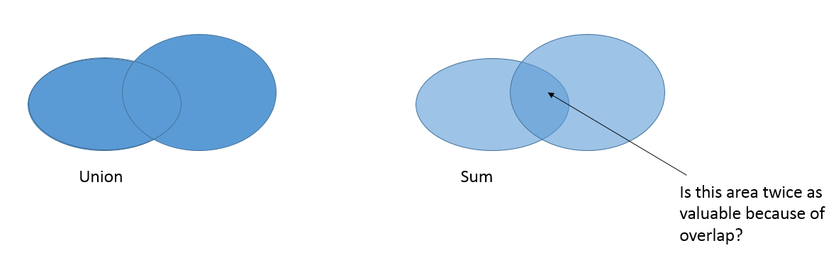
-
Correlate: Data layers that were measured in different units and that were normalized and combined using addition were screened for potential correlation.
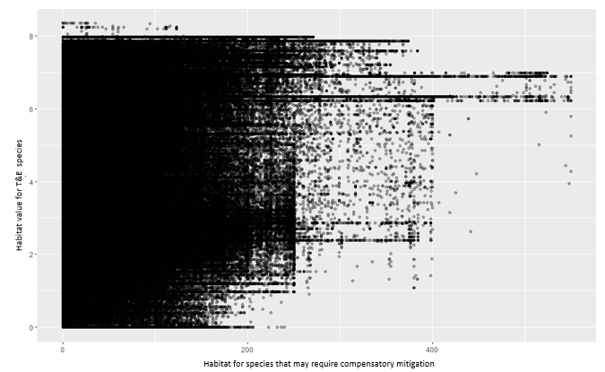
Multi-Benefit Policies
What policies protect riparian corridors?
The following policies protect riparian corridors in the Bay Area.
| Policy | Jurisdiction | Protection |
|---|---|---|
| Biological Resources, Policy 7-1.1.B | Fremont | Assess development within a 100 foot buffer from the top of the riparian bank. Fremont states water conservation is coordinated with Alameda County Water District. Streams are considered a vital water resource protected through irrigation systems and drought tolerant landscaping. |
| Biological Resources, NHR-A.1.3 | Union City | Development of areas within 100 feet of areas. Alongside Alameda County Flood Control natural conditions of streams and creek corridors will be protected. The natural character should be restored and development of trails alongside will be encouraged. |
| Biological Resources Overlay Plan | Alameda County, Castro Valley | 100 feet buffer from of the top of the creek. The city protects natural wildlife via conservation. This will feature open space connected to large habitat areas. Conservation encourages landowners to initiate easements that protects wildlife. |
| Biology and Natural Resources, Policy 4-P-1 | Petaluma | Creation of a 50 foot setback from each bank for Petaluma River and its tributaries; insuring that no development shall occur except for greenway enhancement such trails. Setbacks are increased within significant habitat areas such as wetlands. |
| Benicia General Plan, Visual Character | Benicia | 25 foot buffer dev.prohibited. Grasslands should be protected by creating 25 foot setbacks that no development can be done in. |
| Community Resources and Potential Hazards Plan | Gilroy | Set back development from the entire floodway of the creek, along Uvas Creek and the main branch of Llagas Creek either the entire area of the floodway or 250 feet on either side of the creek centerline, whichever is greater. |
| Conservation Element Plan, Policy 1.3 and 2.7 and 3.1 | Los Altos Hills | Protect, preserve and avoid development on environmentally sensitive resources including creeks and riparian corridors . |
| Conservation Plan, Policy 8-89 | Contra Costa County | 50 ft from riparian buffer. Development that destroys riparian habitats will be held accountable for restoring amount of the habitat destroyed. Setback areas must be specific parameters in order to allow the best maintenance and prevent further damage. |
| Conservation,Design, And Open Space Plan, Policy CDO 7-1 | Cloverdale | 100 ft buffer or more encouraged. Setbacks of 300 - 1,000 feet around the Russian River while tributaries setbacks are encouraged at 50 feet on each side of bank. |
| Conservation Plan, Policy CON-14 and CON-28 | Napa County | 100 foot buffer Development by Permit. When impacts to riparian woodland is infeasible, developers shall be responsible for providing and maintaining a similar replacement habitat. While an on-site location is preferred, the County may approve an off-site location. |
| Creek and Drainageway Setbacks, CON-6 | San Rafael | Maintain a minimum 25 foot development-free setback from the top of creek banks for all new development except for Miller Creek and its tributaries, where a minimum 50 foot setback shall be maintained. |
| Conservation Action RIP-8 | Alameda County | 30 to 100 foot buffer. The EAC Conservation Strategy seeks to preserve endangered species through habitat protection, it acts only as guidance during planning E.G providing mapping system to monitor environmental mitigation measures. |
| Policy 1 Ecology of Creeks and Streams | Novato | 50 foot buffer. Establish a Stream Protection Zone for watercourses with a strip of land extending 50 feet laterally outward from the top of each bank. |
| Environmental Management Plan, Policy EM-2.5 | San Carlos | Riparian policy with 25 foot buffer. Promote the establishment of native vegetation and the removal of nonnative invasive plants in riparian areas. |
| General Plan book B, O-25: R-RC 31,R-RC 32, R-RC 37 and R-RC 38 | Santa Clara County | 100 foot of the top of a creek bank. Keep natural streams, riparian areas,freshwater marshes by protecting from pollution, development impact, hazardous chemicals; adopting tree removal regulations,protecting endemic and endangered species. |
| Stream Conservation Areas, Policy BIO-4.1 | Marin County | 20 foot buffer minimum in city corridor; 100 foot minimum in coastal, baylands corridors; 20 feet minimum in streams. Inside the City-Centered Corridor, a setback from streams is 100 feet for parcels above 2 acres, 50 feet between 0.50 and 2 acres and 20 feet for 1/2 acres. |
| Natural and Historic/Cultural Resources, Policy P8.3.2 | American Canyon | 100 foot buffer. Unless no feasible alternative exists, prohibit developments that alter the biological integrity of riparian corridors. Damaged habitat may be replaced with a habitat of equivalent value. |
| Natural Resources Plan, Riparian Resources Protection NR-1 TO NR-9 | Healdsburg | 100 foot setback from Russian River, 35-foot setback. From Foss Creek, 25-foot setback from other streams. Moreover new development will be located to maximize the riparian vegetation protection. |
| Natural Resources Policy, Stream and Riverbank Protection, NR-1.1 | Napa (city) | 100 foot buffer from waterway. All future waterway projects and projects within 100 feet of a waterway will be reviewed to ensure that they minimize their effects on surrounding habitats. Native plantings are encouraged along waterways to stabilize banks and reduce stormwater runoff. |
| Open space and Conservation Plan, Policy P!0 | Livermore | The city plan restricts development in a riparian corridor which extends, to prohibit the conversion of land, to cultivated agriculture or allowing animals, which reduce the quality of water. |
| Open Space and Conservation Plan, Policy OSC-22 | Tiburon | 50 to 100 foot setback from riparian buffer. An environmental assessment is required for developments proposed on sites that may contain special-status species, sensitive natural communities, native wildlife nurseries and nesting locations. |
| Open Space and Conservation Plan, Policy P8.3‐I‐2 and P8.3-1-3 | San Ramon | 100 foot buffer from riparian centerline. Structures are not to be located within 100 feet of a creek or stream channel as identified on the Zone Map. In addition, a horizontal distance should be considered by a drainage report. |
| Open Space and Conservation, Policy P2.1-2 and P2.1-3 | Calistoga | 30 foot buffer from stream. Developments within a protective stream buffer must include a riparian habitat management plan. Moreover, all waterways shall be buffered to prevent development and preserve open spaces around rivers and streams. |
| Portola Valley Ordinance 2007-369 | Portola Valley | 55 foot from riparian buffer. As an objective quality, where appropriate, enhancing and restoring streams and lesser drainage courses and corridors, unique resources in the regions are the necessity of having the standard open spaces. |
| Sonoma County Ordinance 6089 | Sonoma County | Protect and enhance riparian corridors along streams in order to balance multiple uses. Establishment of streamside conservation areas on both sides of designated riparian corridors ranging 200 feet from Russian River, 100 feet from Flatland and 50 feet from other riparian corridors. |
| Riparian Corridors, Policy OS-30 | Rohnert Park | 100 foot buffer from creeks. Creek protection zones extend at least 50 feet from each bank. Wider buffers are to be established in significant habitat areas. No development in these areas but for greenway enhancement such as trails and bikeways. |
| Policy N-9, Policy N-10, and Policy N-11 | Palo Alto | Apply flood control and public safety measures that preserve the natural environment and habitat of creek; work in collaboration in order to enhance riparian corridors and provide adequate flood control and preserve integrity of riparian corridors. |
| Resource Conservation & Management Plan | Rio Vista | 100 feet for perennial streams, 50 feet from intermittent streams. Depending upon the circumstance and kind of project, appropriate setbacks must be applied to protect sensitive habitats. |
| Resource Implementation Program, RS.I-67 | Solano County | Varying 20, 50, 100, or 150 foot buffer from streams. An ordinance has to be developed that protects riparian water quality through proper buffer zones that keep riparian areas an appropriate width apart from one another depending upon the size of the developed land, respective buffer zones must be set. |
| Riparian Corridors Policies, ER-2.2 | San Jose | 100 foot setback from riparian habitat. Ensure developments are consistent with Riparian Corridor Policy. implement appropriate measures to restore, and/or mitigate damage; update Policy; restrict or carefully regulate development in streamside. |
| Santa Clara County Habitat Conservation Plan, Riparian policy | Santa Clara County | 150 to 200 foot riparian buffer. Main goal of HCP is to gain authorization for incidental take of covered species under the ESA and the NCCP Act for activities which will occur in accordance with approved land-use and capital-improvement plans. |
| Sensitive Habitat, Riparian Corridor, Policy 7.11 | San Mateo County | Local Coastal Plan 50 foot buffer, 30 feet for intermittent streams. Develop guidance for Vegetation control in Riparian Corridors should set 4th direction on procedures to decrease flood threats and an award must be given to the responsible corridor managers. |
Methods: The jurisdictional policies adopted that reduce impacts from urban development on riparian corridors are reviewed and digitally rendered based upon jurisdictions’ general plans and zoning maps. With the exception of Sonoma County and Santa Clara County HCP Riparian Corridors available online, the remaining policies were calculated with a buffer corresponding to their policy language against the centerline of the USGS National Hydrography Dataset’s Flowline.
What policies protect ridges and hillsides?
The following policies protect hillside areas in the Bay Area.
| Policy | Jurisdiction | Protection |
|---|---|---|
| Residential communities design principles: Policy 1.11.7b | American Canyon | Require developments to preserve the topographic character of hillsides and canyons by concentrating projects on lesser slopes, no mass grading on slopes exceeding 25 percent. |
| Residential communities design principles: Policy 1.11.7c | American Canyon | Prohibit development on slopes exceeding 50 percent and maintenance of natural grades in higher elevation areas. |
| Open Space and conservation of resources | Benicia | Hillside areas that have slope over 30 percent are to be kept as open space areas. |
| Environmental protection: Ordinance 19.08.040 Slope regulations. | Calistoga | No construction, grading or vegetation removal may occur in areas with a slope of 30 percent or greater, unless an exemption is granted. Permitted projects are subject to restrictions and design reviews related to their location. |
| Land use element: Policy LU 3-2 Implementation LU 3-2.a. | Cloverdale | Within urban growth boundaries, apply a hillside ordinance restricting development for any areas above 400 feet elevation and for properties over 20 percent slope. |
| Scenic resources policies: Policies 9-14 and 9-21 | Contra Costa County | By using zoning measures amongst other appropriate measures, hillsides with a slope of 26 percent or greater will be not be constructed upon. Additionally, there should be no construction within 50 feet or on top of major scenic ridgelines. |
| Residential hillsides-site development regulations: Ordinance 19.40.050, H. Development Neart Prominent Ridgelines, I. Development on Slopes ≥ 30% | Cupertino | Construction or improvements of structures limited in specific hillsides include keeping 15 percent site line from a prominent ridge, and hillside exception required for development with greater than 500 square feet area on slopes equal or greater than 30 percent. |
| Uses and Development of Lands Identified as Scenic Hillside or Major Ridgeline Areas: Ordinance 32-69.4 | Danville | No construction of buildings will be done on areas of land 100 feet below the centerline of a ridgeline or on a slope of less than 30 percent in steepness. |
| Erosion and Siltation control: Implementing policies 3 | Dublin | Restrict development on slopes over 30 percent. |
| Residential uses: Policy 26 | Alameda County | In no case shall required housing be built on or which protrudes over hilltops or ridgelines, on slopes of more than 20 percent critical wildlife habitat, or within 100 feet of a riparian corridor. |
| Ridgeline development : Ordinance 17.060:050 | Fairfax | Developments within 100 vertical feet or 150 horizontal feet of a major scenic ridgeline requires additional permitting. |
| Health and Safety Element: Policy HS 2.4 | Fairfield | Measure T permits only very low densities of one unit per 20 acres for existing parcels. |
| Hill Area Open Space | Fremont | The Hill Area Open Space designation applies to most of the open lands defined by voter-approved Measure A (Hillside Initiative of 1981) and Measure T (Hill Area Initiative of 2002). |
| Measure A: Hillside Open Space | Fremont | Measure A prevents land from exceeding one unit per acre or one unit per four acres for constrained lands. |
| Measure T:Hill face open space | Fremont | Measure T permits only very low densities of one unit per 20 acres for existing parcels. |
| Slope Restrictions: Policy 25.11 | Gilroy | Slopes of 10 to 30 percent may be suitable for low intensity, low density development, subject to site-specific review and approval. |
| Slope Restrictions: Policy 25.11 | Gilroy | Slopes greater than 30 percent, areas of high landslide risk, and areas with highly expansive soils on slopes greater than 10 percent are not suitable for development and will remain open space. |
| Hillside development: Policy LU-7.1 | Hayward | The city will protect hillside areas, retaining natural slopes and sensitive areas. This involves protection of slopes, which are deemed unstable such as those greater than 25 percent. |
| Development restriction on class I or II ridgeline: ordinance 6-2023 | Lafayette | Major ridgelines are to be preserved in their natural state as a natural resource and wildlife corridor A setback of 400 feet for a Class I ridgeline and a setback of 250 feet for a Class II ridgeline should be implemented. |
| Open space: Policy b | Larkspur | Designate lands above 350 feet in the Northridge area of Larkspur as open space. |
| Protect and preserve open space: Policy 1.2-program 1.2 | Los Altos | Leave intact and put requirements to set aside of development generally on areas in excess of 30 percent hillside slope. |
| Ridge and Upland Greenbelt: Program DES-4.e | Marin County | Protect views of the Ridge and Upland Greenbelt Areas by amending policies and maps to identify a border on parcels that abut the area. Developments are to adhere to requirements that include visually sensitive designs and rural densities. |
| Open space preservation: Policy OS1.5 | Moraga | Development is prohibited if the slope on the ridge is greater than 20 percent and if the elevation of the ridge is more than 800 feet. |
| Preservation of hillside areas as open space: Action 4.5 | Morgan Hill | Hillside Ordinance should be applied for a development on areas with an average slope in excess of 10 percent. |
| Hillside combining district-Building restriction: Ordinance 18.44.030. | Morgan Hill | No construction allowed on areas greater than 20 percent with exception of development proposal that is not conflicted with this policy. |
| Preservation of hillside areas as open space: Action 4.1 | Morgan Hill | Preserve El Toro Mountain in open space above the 500 foot contour line on all sides, with the exception of the Llagas and Paradise Valleys where all land above the 600 foot contour elevation should be preserved. |
| Preservation of hillside areas as open space: Action 4.1 and 4.5 | Morgan Hill | Hillside Ordinance should be applied for a development on areas with an average slope in excess of 10 percent while construction is not allowed on area greater than 20 percent slope. Preserve El Toro Mountain at an elevation above 500 feet and Llagas and Paradise Valleys above 600 feet. |
| Preservation of hillside areas as open space: Action 4.1 | Morgan Hill | Hillside Ordinance should be applied for a development on areas with an average slope in excess of 10 percent while construction is not allowed on area greater than 20 percent slope. Preserve El Toro Mountain at an elevation above 500 feet and Llagas and Paradise Valleys above 600 feet. |
| Preservation of hillside areas as open space: Action 4.1 and 4.5 | Morgan Hill | Hillside Ordinance should be applied for a development on areas with an average slope in excess of 10 percent while construction is not allowed on area greater than 20 percent slope. Preserve El Toro Mountain at an elevation above 500 feet and Llagas and Paradise Valleys above 600 feet. |
| Preservation of hillside areas as open space: Action 4.1 and 4.5 | Morgan Hill | Hillside Ordinance should be applied for a development on areas with an average slope in excess of 10 percent while construction is not allowed on area greater than 20 percent slope. Preserve El Toro Mountain at an elevation above 500 feet and Llagas and Paradise Valleys above 600 feet. |
| View protection program: Structures and Related improvements | Napa County | Administrative approval might be granted if the average slope of each development area is less than 30 percent. |
| View protection program: Structures and Related improvements | Napa County | For an area with the average slope of any development 30 percent or greater, work in that area cannot be undertaken unless a use permit is approved by the Napa County Zoning Administrator or Conservation Development and Planning Commission. |
| Hillside Project Development Standards: Ordinance 19.26.050 | Novato | No development potential shall be allowed for areas with average slopes of greater than 25 percent. |
| Natural Hazards: Policy 10-P-1 B | Petaluma | On sites with slopes greater than 30 percent, require all development to be clustered outside of the 30 percent slope areas, and preferably on land less than 15 percent in slope, where possible. |
| Regional Open Space Preserves: Policy OS.6.3 | Pinole | Preserve major and minor ridgelines. Where possible, properties shall provide for a ridgeline setback of 400 feet horizontally from major ridgelines, 100 feet from minor ridgelines and a vertical setback of 100 feet from both. |
| Hillside protection: Policy 9-P-6 | Pittsburg | Building pads and structural elements shall be located at least 150 feet away, horizontally, from the crest of a major ridgeline. |
| Measure PP: Ridgelines and Hillsides protection | Pleasanton | Placing housing units or structures on slopes of 25 percent or greater or within 100 vertical feet of a ridgeline is prohibited. |
| Program 21.3-Ridgelines and Hillsides protection | Pleasanton | Placing housing units or structures on slopes of 25 percent or greater or within 100 vertical feet of a ridgeline is prohibited. |
| Open Space element: Principle 14 | Portola Valley | Areas including with slopes generally over 30 percent hazardous to the public safety and welfare should be retained as open space. |
| Protection of ridges: Policy 2.7 | San Anselmo | The ridge zone shall extend 150 horizontal feet in both directions from the lowest elevation of the ridgeline, or 50 feet vertically, whichever is more restrictive. Development prohibited on land with an elevation above 150 feet. |
| Single-Family Residential-Conservation | San Anselmo | Development prohibited on land with an elevation above 150 feet and should be protected and placed in a special conservation zone. |
| Single-Family Residential-Conservation and Protection of ridges: Policy 2.7 | San Anselmo | The ridge zone shall extend 150 horizontal feet in both directions from the lowest elevation of the ridgeline, or 50 feet vertically, whichever is more restrictive. |
| Hillside and Rural Preservation: Policy LU-17.6 | San Jose | No development allowed along ridges and other major hillside areas with slope greater than 30 percent. |
| Local Coastal Program (LCP) | San Mateo County | Review development proposals in designated hazardous areas and regulation of development on 30 percent or steeper slopes prior to issuance of any development permit. |
|
Hillside, Creek, and Ridgeline Area Development Standards : 4. Ridgeline setback |
San Ramon | No structure will be located within 100 feet of a major ridgelines and 50 feet of minor ridgelines. |
| Development on steep slopes: Policy R-GD 29 | Santa Clara County | Development initiatives on areas greater than 30 percent slope shall thoroughly evaluated before approval in accordance with all existing regulations. In addition, a public hearing shall be required, and notice should be provided within 300 feet of the subject property |
| Open space: Policy OSC-B-5 | Santa Rosa | Require a Hillside Development Permit under certain development conditions where a portion of the site has a slope greater than 10 percent. |
| Site grading: Policy 10 | Saratoga | Construction is not allowed in an area with an average slope that exceeds 30 percent or an area that exceeds 40 percent natural slope under the structure. Additional requirement must be consistent the Measure "A" area, or hillside specific plan. |
| Policy for reduction of soil erosion- Policy OSRC-11a and Policy OSRC-11b | Sonoma County | Design discretionary projects so that structures and roads are not located on slopes of 30 percent or greater. Include erosion control measures for any discretionary project involving construction or grading on lands with slopes over 10 percent. |
| Scenic landscape unit: Policy OSRC-2a | Sonoma County | Avoid amendments to increase residential density in Scenic Landscape Units in excess of one unit per ten acres. The land use plan may designate a lower density or larger minimum lot size. |
| Ridgeline policies: Policy OSC-10 and OSC-11 | Tiburon | When considering open space and development interests, undeveloped ridgelines are to have the highest priority. Developments and landscaping shall be setback a minimum of 150 horizontal feet and 50 vertical feet of either side of Tiburon Ridge. |
| Development clustering: Policy 8 | Union City | Development clusters which are concentrated areas of development surrounded by open space buffers shall be encouraged in the Hillside Area. |
| Policy LU-P24.1 | Vacaville | Areas with ridges and slopes of 25 percent or greater should stay undeveloped in order to keep agricultural areas intact. |
| Hillside development Policy 2 | Vallejo | Projects for building in Planned Development areas which have natural slopes exceeding 10 percent will be evaluated in order to make sure that the natural lay of the land is kept. |
| General plan protection open space | Walnut Creek | The development of land with slopes of 20 percent or greater or within 75 vertical feet of any ridgeline is prohibited. |
| Policy A.1.1 | Windsor | Developments proposed on slopes greater than 20 percent will require assessment of stability. |
Methods: Hillside areas identified as important for protection or to minimize landslide threat are based upon the physical descriptions in city and county general plans. Policies are mapped using a digital elevation model to assess the slope of a hill, the area of a hill above a certain elevation, and the area within a certain vertical or horizontal distance from a ridge line. The slope is calculated as slope percent rise, an elevation area is selected above the lowest limit of the defined elevation, horizontal distance from the ridge is calculated using a buffer, while vertical distance from a ridge is calculated from the elevation data as a vertical drop relative to the height of the closest point on the ridgeline.
What policies protect general conservation values?
The following policies protect general conversation values in the Bay Area.
| Policy | Jurisdiction | Protection |
|---|---|---|
| Concord Reuse Project, Conservation Open Space | Concord | The Concord Reuse Project site will have portions of its land that are considered open space and thus should be protected accordingly. |
| Dublin Open Space Initiative 2014 | Dublin | The provisions of the Dublin Open Space Initiative of 2014 should be carried out and enforced diligently and effectually and uses and the location, amount, visibility, and environmental effects of all proposed development should be reviewed. |
| Open Space Reserve | Half Moon Bay | The city has designated portion of areas as open space reserve consistent with the policy of the Coastal Act; including areas currently in some form of agricultural use and areas not now in production. These areas will not be converted to urban uses. |
| Franklin Canyon (Measure M) | Hercules | The purpose of this ordinance is to protect Franklin canyon and nearby open space lands from harmful and unnecessary development. |
| Morgan Hill Greenbelt | Morgan Hill | Greenbelt, to demarcate and distinguish urban area of Morgan Hill; located outside of ULL; include areas with steep hillside, severe geologic/environmental constraints, open space & located on the fringe of the community & not include unincorporated areas. |
| Sensitive Local Resource Areas | Rio Vista | It should be ensured that the development process respects the unique characteristics and functions of Sensitive Local Resource Areas including avoidance of disturbance; on-site restoration and in-kind restoration. |
| San Jose: Coyote Valley Greenbelt | Morgan Hill | Work in collaboration with the City of San Jose and Santa Clara County in order to ensure the San Jose Coyote Valley Greenbelt continues providing the non-urban buffer for the north side of Morgan Hill. |
| Cooperative Planning Area for Agriculture and Open Space | Solano County | Cooperative plan for agriculture and open space preservation intends to establish permanent open space between the cities of Benicia, Fairfield and Vallejo mutual agreement of a cooperative planning area for agriculture and open space. |
| Davis-Dixon Greenbelt | Dixon, Davis , the Solano Land Trust, federal and state agencies | Permanently protecting the prime farmlands and scenic resources of the area located between the two cities. |
| Resource Conservation Overlay | Solano County | Solano's Resource Conservation identifies and protects areas of the county with special resource management needs. |
| Vacaville-Dixon Greenbelt | Vacaville-Dixon Greenbelt Authority | Guarantee that certain lands located between the two cities remains an agricultural landscape in perpetuity. It is implemented through acquisition from willing sellers and resale of the properties with a permanent conservation easement |
| Vacaville-Fairfield-Solano Greenbelt | Vacaville Fairfield-Solano Greenbelt Authority | Permanent, one-mile-wide, open space greenbelt that serves as a community separator, a setting for recreational activities, a buffer between agricultural and urban areas, and as an ultimate limit for urban growth. |
| Community Separators | Sonoma County | Preserve the visual identities of communities by maintaining open space areas (Community Separators) between cities and communities. |
Methods: The jurisdictional policies adopted that reduce impacts on important conservation values from urban development are reviewed and digitally rendered based upon jurisdictions’ general plans.
Multi-Benefit Conservation Assessment
The multi-benefit conservation assessment maps the degree of overlap of nature's values and benefits. Darker areas have more overlap of natural and/or agricultural resources. A widget that controls the map empowers users to make all decisions about weighting and combining multi-benefit information by allowing users to select which values or benefits are included and to adjust the relative influence of each value or benefit.
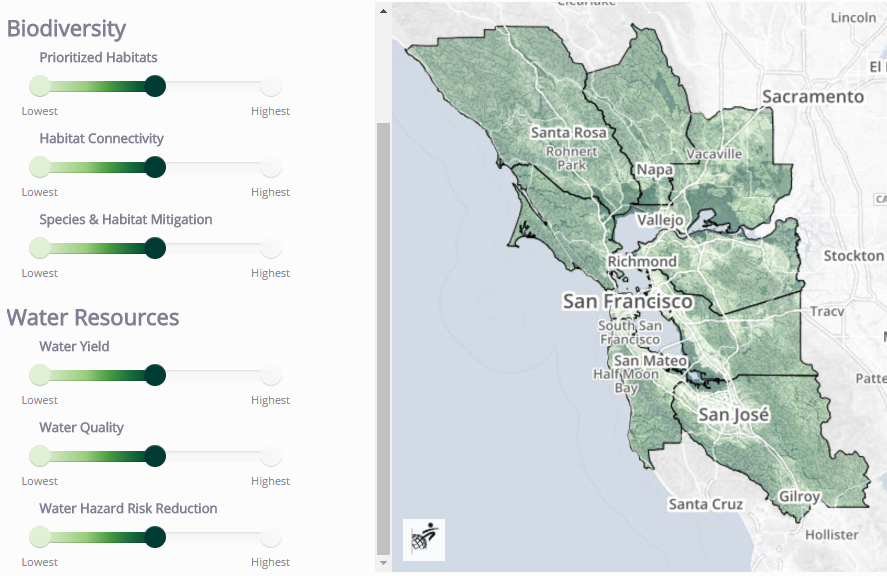
Why is it useful?
The user-defined multi-benefit assessment:
Methods
The building blocks of the multi-benefit conservation assessments are individual assessments for each of the nine nature's values or benefits. Each individual assessment is built from the 2-5 data layers listed below. These data layers correspond with the metrics in the Greenprint Report which are displayed in tabular format for each value or benefit.
Results
The final conservation assessments for each of the nine nature's values and benefits are shown below.